Chapter 4 Lab 2 - 10/03/2022
In this lecture we will learn how to import data from an external file, how to deal with data frames. Moreover, we will use the main functions of the tidyverse package.
4.1 Data import
We have some financial data (about loan default) available in the csv file named Default_Fin.csv. Note that a csv file can be open using a text editor (e.g. TextNote, TextEdit), see Figure 4.1.
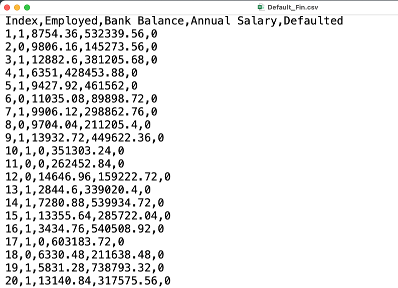
Figure 4.1: Preview of the csv file
There are 3 things that characterize a csv file:
- the header: the first line containing the names of the variables;
- the field separator (delimiter): the character separating the information (usually the semicolon or the comma is used);
- the decimal separator: the character used for real number decimal points (it can be the full stop or the comma).
In the preview of the csv file reported in Figure 4.1
- the header is given by a set of text strings:
- “,” is the field separator;
- “.” is the decimal separator.
All this information are required when importing the data in R by using the read.csv function, whose main arguments are reported here below (see ?read.csv):
file: the name of the file which the data are to be read from; this can also including the specification of the folder path (use quotes to specify it);header: a logical value (TorF) indicating whether the file contains the names of the variables as its first line;sep: the field separator character (use quotes to specify it);dec: the character used in the file for decimal points (use quotes to specify it).
The following code is used to import the data available in the Default_Fin.csv file. The output is an object named defdata:
defdata <- read.csv("./files/Default_Fin.csv")The argument sep=",", header=T and dec="." are set to the default value (see ?read.csv) and they could be omitted.
Alternatively, it is possible to use the user-friendly feature provided by RStudio: read here for more information. The data import feature can be accessed from the environment (top-right) panel (see Figure 4.2). Then all the necessary information can be specified in the following Import Dataset window as shown in Figure 4.3.
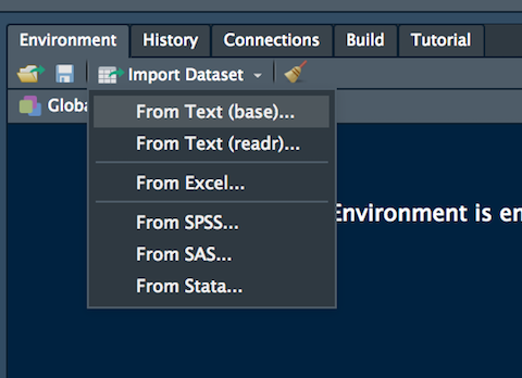
Figure 4.2: The Import Dataset feature of RStudio
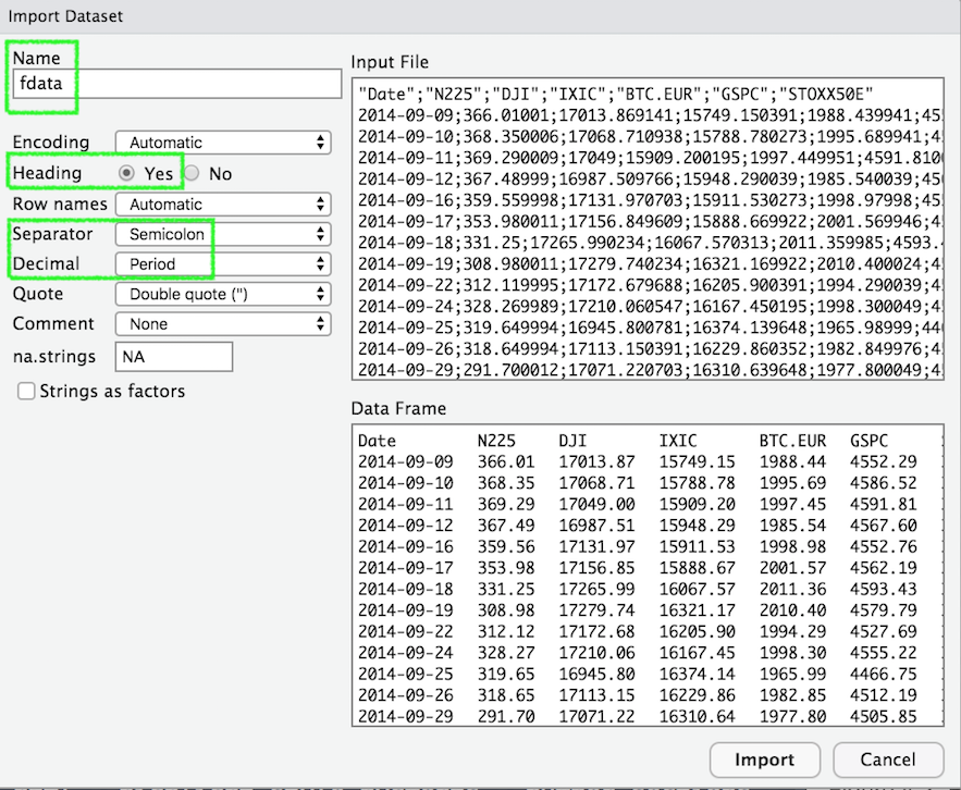
Figure 4.3: Specification of the csv file characteristics through the Import Dataset feature
After clicking on Import an object named defdata will be created (essentially this RStudio feature makes use of the read.csv function).
The defdata is an object of class data.frame:
class(defdata)## [1] "data.frame"Data frames are matrix of data where you can find statistical units in the rows and variables in the column (in this case you have the following variables: Index, Employed, Bank.Balance, etc.).
By using str we get information about the type of variables included in the data frame:
str(defdata)## 'data.frame': 10000 obs. of 5 variables:
## $ Index : int 1 2 3 4 5 6 7 8 9 10 ...
## $ Employed : int 1 0 1 1 1 0 1 0 1 1 ...
## $ Bank.Balance : num 8754 9806 12883 6351 9428 ...
## $ Annual.Salary: num 532340 145274 381206 428454 461562 ...
## $ Defaulted. : int 0 0 0 0 0 0 0 0 0 0 ...In this case all the variables are in the form of (integer or real) numerical variables.
It is possible to get a preview of the top or bottom part of the data frame by using head or tail:
head(defdata) #preview of the first 6 lines (oldest data)## Index Employed Bank.Balance Annual.Salary Defaulted.
## 1 1 1 8754.36 532339.56 0
## 2 2 0 9806.16 145273.56 0
## 3 3 1 12882.60 381205.68 0
## 4 4 1 6351.00 428453.88 0
## 5 5 1 9427.92 461562.00 0
## 6 6 0 11035.08 89898.72 0tail(defdata) #preview of the last 6 lines (most recent data)## Index Employed Bank.Balance Annual.Salary Defaulted.
## 9995 9995 0 2068.92 179471.3 0
## 9996 9996 1 8538.72 635908.6 0
## 9997 9997 1 9095.52 235928.6 0
## 9998 9998 1 10144.92 703633.9 0
## 9999 9999 1 18828.12 440029.3 0
## 10000 10000 0 2411.04 202355.4 0Use the following alternative function if you want to get information about the dimensions of the data frame:
nrow(defdata) #number of rows## [1] 10000ncol(defdata) #number of columns## [1] 5dim(defdata) #no. of rows and columns## [1] 10000 54.2 Data selection from a data frame
To select data it is possible to use squared parentheses as seen in Lab 1 for vectors, but in this case two indexes (one for the row and one for the column) will have to be specified.
For example the code
defdata[1,3] #first number is the row index, the second is the column index## [1] 8754.36is used to retrieve the element in the first row and third column, corresponding to the bank balance value the first observation.
If more elements together are requested, a vector of indexes can be used. Here we extract the first 5 statistical units and the third and fourth variables:
defdata[ 1:5 , 3:4]## Bank.Balance Annual.Salary
## 1 8754.36 532339.6
## 2 9806.16 145273.6
## 3 12882.60 381205.7
## 4 6351.00 428453.9
## 5 9427.92 461562.0To select an entire row (i.e. all the information for a given statistical unit) you have to specify only the row index:
defdata[1,] #all the information for the 1st observation## Index Employed Bank.Balance Annual.Salary Defaulted.
## 1 1 1 8754.36 532339.6 0Similarly, if you are interested in a particular column (i.e. all the values/categories for a given variable), specify only the column index
head(defdata[,2]) ## [1] 1 0 1 1 1 0#all the values for Employed (short preview with head)or alternatively perform the selection by using the $ followed by the column name:
head(defdata$Employed) ## [1] 1 0 1 1 1 0#all the values for Employed (short preview with head)
#this is a vector (one dimensional object)Given a vector it is then possible to select an element by using the one dimensional index. Select for example the first value of the vector defdata$Employed:
defdata$Employed[1]## [1] 1This is equivalent to
defdata[1,2]## [1] 1Note that the Employment variable is so far considered as a binary quantitative variable. It is thus possible to use sum and mean to compute the number and percentage of employment people, as shown in Lab 1:
sum(defdata[,2])## [1] 7056mean(defdata[,2])*100## [1] 70.56It is also possible to get the frequency distribution using the function table (showing the number of people for each category):
table(defdata$Employed) ##
## 0 1
## 2944 70564.3 Factor
A factor object is used to define categorical (nominal or ordered) variables. It can be viewed as integer vectors where each integer value has a corresponding a label. It’s more convenient than a vector of characters as each unique character value is stored only once, and the data itself is stored as a vector of integers.
Let’s first of all simulate some values by sampling 10 values between 1 and 5:
set.seed(155)
x = sample(1:5, 10, replace = TRUE)
x
## [1] 2 1 2 1 4 4 2 2 2 2Let’s assume now that these values are actually categories of a categorical variable, e.g. 1 could be “definitely no” and 4 “definitely yes”. We define the factor as follows:
xf = factor(x)
xf
## [1] 2 1 2 1 4 4 2 2 2 2
## Levels: 1 2 4levels(xf)## [1] "1" "2" "4"Note that a factor is defined by its levels which by default are given by the observed values. But we know that the values are sampled from 1:5 and thus the possible categories are the integers between 1 and 5. So create accordingly a new object:
xf2 = factor(x, levels = 1:5)
xf2
## [1] 2 1 2 1 4 4 2 2 2 2
## Levels: 1 2 3 4 5class(xf2)## [1] "factor"It is possible to set a different label for each levels, as follows:
xf3 = factor(x, levels = 1:5,
             labels = c("def.not",
                        "not",
                        "I don't know",
                        "yes",
                        "def.yes"))
xf3
## [1] not def.not not def.not yes yes not not not
## [10] not
## Levels: def.not not I don't know yes def.yesclass(xf3)## [1] "factor"It is also worth to note that the categories in this case are ordered, thus we can define a new object by taking this into account:
xf4 = factor(x, levels = 1:5,
             labels = c("def.not",
                        "not",
                        "I don't know",
                        "yes",
                        "def.yes"),
             ordered = T)
xf4
## [1] not def.not not def.not yes yes not not not
## [10] not
## Levels: def.not < not < I don't know < yes < def.yesclass(xf4)## [1] "ordered" "factor"In this case it is possible to check if the first observation has expressed an opinion lower (more negative) than the second unit. The following computation is possible only because the factor is ordered:
xf4[1] < xf4[2]## [1] FALSEIf the factor is not ordered it is possible only to check == or != conditions, e.g.:
xf2[1] != xf2[2]## [1] TRUEComing back to the defdata dataframe we are going to transform the variables Employed and Defaulted into factors as we know that they are actually categorical variables (coded with 0/1):
defdata$Employed = factor(defdata$Employed,
       levels = c(0,1),
       labels = c("Not Employed", "Employed"))
head(defdata)
## Index Employed Bank.Balance Annual.Salary Defaulted.
## 1 1 Employed 8754.36 532339.56 0
## 2 2 Not Employed 9806.16 145273.56 0
## 3 3 Employed 12882.60 381205.68 0
## 4 4 Employed 6351.00 428453.88 0
## 5 5 Employed 9427.92 461562.00 0
## 6 6 Not Employed 11035.08 89898.72 0table(defdata$Employed)##
## Not Employed Employed
## 2944 7056defdata$Defaulted = factor(defdata$Defaulted,
levels = c(0,1),
labels = c("Not Defaulted", "Defaulted"))
head(defdata)## Index Employed Bank.Balance Annual.Salary Defaulted. Defaulted
## 1 1 Employed 8754.36 532339.56 0 Not Defaulted
## 2 2 Not Employed 9806.16 145273.56 0 Not Defaulted
## 3 3 Employed 12882.60 381205.68 0 Not Defaulted
## 4 4 Employed 6351.00 428453.88 0 Not Defaulted
## 5 5 Employed 9427.92 461562.00 0 Not Defaulted
## 6 6 Not Employed 11035.08 89898.72 0 Not Defaultedtable(defdata$Defaulted) #unbalanced distribution ##
## Not Defaulted Defaulted
## 9667 3334.4 Install and load a package
A R package is a collection of R functions, complied code and sample data. It can be considered as an extension of the base R release.
tidyverse is a package which is actually a collection of R packages designed specifically for data science (see Figure 4.4). All the packages share an underlying design
philosophy, grammar, and data structures. See here for more details.

Figure 4.4: Packages included in tidyverse
The tidyverse-based functions process faster than base R
functions. It is because they are written
in a computationally efficient manner and are
also more stable in the syntax and better supports
data frames than vectors.
Before starting using a package it is necessary to follow two steps, depicted in Figure 4.5:

Figure 4.5: Install and load a R package
- install the package: this has to be done only once (unless you re-install R, change or reset your computer). It is like buying a light bulb and installing it in the lamp, as described in the left panel of Figure 4.5: you do this only once not every time you need some light in your room. This step can be performed by using the RStudio menu, through Tools - Install package, as shown in Figure 4.6. Behind this menu shortcut, RStudio is using the
install.packagesfunction.
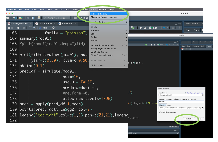
Figure 4.6: The Install Package feature of RStudio
- load the package: this is like switching on the light one you have an installed light bulb, something that can be done every time you need some light in the room (see the right panel in Figure 4.5). Similarly, each package can be loaded whenever you need to use some functions included in the package. For example to load the
tidyversepackage we proceed as follows:
library(tidyverse)Once the tidyverse package is loaded, we are ready to use all the functions contained in the package.
4.5 The pipe operator
Let’s consider a general R function named f with argument x. We usually
use the following approach when we need to apply f:
f(x)An alternative is given by the pipe operator %>% which is part of the
dplyr package (see here for more details). It works as follows
x %>% f()
#this is equivalent to f(x)
Basically, the pipe tells R to pass x as the first argument of the function f. The shortcut to type the pipe operator in RStudio is given by CTRL/CMD Shift M.
We are for example interested in computing the natural log transformation of the value 4. By adopting the standard R programming we would use:
log(4)## [1] 1.386294while with the pipe operator we have
4 %>% log()## [1] 1.386294#it's also possible to omit the parentheses given that there is no inputwhere 4 is taken as the first argument of the function log. It is also possible to include other arguments, such as for example the base of the logarithm (in this case equal to 5). In this case note that 4 %>% f(y) is equivalent to f(x,y).
#standard programming
log(4, base=5)
## [1] 0.8613531#pipe based programming
4 %>% log(base=5)## [1] 0.8613531Let’s consider now the vector x given by the first 5 values of the Bank Balance in defdata:
x = defdata$Bank.Balance[1:5] We want now to apply the log transformation and then round the corresponding output to 2 digits. This requires the use of two functions (log and round). In general, when we apply 3 functions (f and then g and finally h), we have that x %>% f %>% g %>% h is equivalent to h(g(f(x))).
# standard programming
round(log(x), 2)
## [1] 9.08 9.19 9.46 8.76 9.15# pipe based programming
x %>% log %>% round(2)## [1] 9.08 9.19 9.46 8.76 9.15We now add a new function: after rounding the log output we compute the sum of the 5 numbers
# standard programming
sum(round(log(x),2))
## [1] 45.64# pipe based programming
x %>% log %>% round(2) %>% sum ## [1] 45.64When it is not convenient to use the pipe:
- when the pipes are longer than 10 steps. In this case the suggestion is to create intermediate objects with meaningful names (that can help understanding what the code does);
- when you have multiple inputs or outputs (e.g. when there is no primary object being transformed but two or more objects being combined together).
4.6 dyplyr verbs
dplyr (a package in the tidyverse collection) is a grammar of data manipulation, providing a consistent set of
verbs that help you solve the most common data manipulation challenges:
select: pick variables (columns) based on their namesfilterpick observations (rows) based on their valuesmutate: add new variables that are functions of existing variablessummarise: reduce multiple values down to a single summary (e.g. mean)arrange: change the ordering of the rows
All verbs work similarly:
- the first argument is a data frame;
- the subsequent arguments describe what to do with the data frame using the variable names (without quotes);
- the result is a new data frame.
In the following we will take into account all the dplyr verbs by considering
the defdata data frame
To get the list and the type of variables included in defdata we can use the standard str or the corresponding tidyverse function named glimpse:
str(defdata)## 'data.frame': 10000 obs. of 6 variables:
## $ Index : int 1 2 3 4 5 6 7 8 9 10 ...
## $ Employed : Factor w/ 2 levels "Not Employed",..: 2 1 2 2 2 1 2 1 2 2 ...
## $ Bank.Balance : num 8754 9806 12883 6351 9428 ...
## $ Annual.Salary: num 532340 145274 381206 428454 461562 ...
## $ Defaulted. : int 0 0 0 0 0 0 0 0 0 0 ...
## $ Defaulted : Factor w/ 2 levels "Not Defaulted",..: 1 1 1 1 1 1 1 1 1 1 ...glimpse(defdata)## Rows: 10,000
## Columns: 6
## $ Index <int> 1, 2, 3, 4, 5, 6, 7, 8, 9, 10, 11, 12, 13, 14, 15, 16, 1…
## $ Employed <fct> Employed, Not Employed, Employed, Employed, Employed, No…
## $ Bank.Balance <dbl> 8754.36, 9806.16, 12882.60, 6351.00, 9427.92, 11035.08, …
## $ Annual.Salary <dbl> 532339.56, 145273.56, 381205.68, 428453.88, 461562.00, 8…
## $ Defaulted. <int> 0, 0, 0, 0, 0, 0, 0, 0, 0, 0, 0, 0, 0, 0, 0, 0, 0, 0, 0,…
## $ Defaulted <fct> Not Defaulted, Not Defaulted, Not Defaulted, Not Default…4.6.1 Verb 1: select
This verb is used to select some of the columns by name. For example, to select the variables Employed and Defaulted we use the following code:
defdata %>%
  select(Employed, Defaulted) %>%
  head() #preview
## Employed Defaulted
## 1 Employed Not Defaulted
## 2 Not Employed Not Defaulted
## 3 Employed Not Defaulted
## 4 Employed Not Defaulted
## 5 Employed Not Defaulted
## 6 Not Employed Not DefaultedIt is also possible to specify a criterion which excludes from the selection some variables. For example, to select all the columns but Index we use the - symbol:
defdata %>%
  select(-Index) %>%
  head() #preview
## Employed Bank.Balance Annual.Salary Defaulted. Defaulted
## 1 Employed 8754.36 532339.56 0 Not Defaulted
## 2 Not Employed 9806.16 145273.56 0 Not Defaulted
## 3 Employed 12882.60 381205.68 0 Not Defaulted
## 4 Employed 6351.00 428453.88 0 Not Defaulted
## 5 Employed 9427.92 461562.00 0 Not Defaulted
## 6 Not Employed 11035.08 89898.72 0 Not DefaultedIt is also possible to create a new data frame that contains only the selected variables:
defdata2 = defdata %>%
  select(-Index)
4.6.2 Verb 2: filter
The verb filter can be used to select the observations satisfying some criterion. Consider the example the selection of defaulted observations in defdata:
defdata2 %>%
  filter(Defaulted == "Defaulted") %>%
  head() #preview
## Employed Bank.Balance Annual.Salary Defaulted. Defaulted
## 1 Not Employed 17844.00 214252.8 1 Defaulted
## 2 Not Employed 26469.60 171257.9 1 Defaulted
## 3 Not Employed 21296.28 244314.1 1 Defaulted
## 4 Employed 22675.20 587474.0 1 Defaulted
## 5 Not Employed 22792.68 247862.4 1 Defaulted
## 6 Not Employed 18874.32 179162.2 1 DefaultedIt is also possible to include more conditions. Select for example the defaulted defdata and with a salary lower than 150000 (the AND can be specified by using &):
defdata2 %>%
  filter(Defaulted == "Defaulted" & Annual.Salary<150000)
## Employed Bank.Balance Annual.Salary Defaulted. Defaulted
## 1 Not Employed 16827.24 145251.8 1 Defaulted
## 2 Not Employed 27994.56 141242.8 1 Defaulted
## 3 Not Employed 17915.52 132648.8 1 Defaulted
## 4 Not Employed 20494.92 127100.6 1 Defaulted
## 5 Not Employed 20177.76 121863.8 1 Defaulted
## 6 Not Employed 22835.64 149571.6 1 Defaulted
## 7 Not Employed 24800.40 125647.7 1 Defaulted
## 8 Not Employed 22727.28 148789.4 1 Defaulted
## 9 Not Employed 21683.04 138074.6 1 Defaulted
## 10 Not Employed 29538.12 142542.7 1 Defaulted
## 11 Not Employed 25405.44 145721.6 1 Defaulted
## 12 Not Employed 24462.48 146182.8 1 Defaulted
## 13 Not Employed 24295.92 115965.5 1 Defaulted4.6.3 Verb 4: summarise
This verbs can be used to compute summary statistics. For example the following code computes the mean and median of Bank.Balance and Annual.Salary:
defdata2 %>%
  summarise(mean(Bank.Balance),
            median(Annual.Salary))
## mean(Bank.Balance) median(Annual.Salary)
## 1 10024.5 414631.7The output is automatically labelled but it is also possible to specify different labels as follows:
defdata2 %>%
  summarise(mean_BB = mean(Bank.Balance),
            median_AS = median(Annual.Salary))
## mean_BB median_AS
## 1 10024.5 414631.7Similarly, it is possible to compute some summary statistics on a new variable which is a transformation of the variables originally contained in the data frame. For example, we are interested in the mean of a new variable given by the monthly salary :
defdata2 %>%
  summarise(mean_MS = mean(Annual.Salary/12))
## mean_MS
## 1 33516.98Another transformation of the original variables consists in considering if an observation is Defaulted or not (T or F) and then computing how many observations (absolute frequency, proportion or percentage) satisfy the condition. This is computed by using the sum or mean functions:
defdata2 %>%
  summarise(sumdef = sum(Defaulted == "Defaulted"),
            percdef = mean(Defaulted == "Defaulted")*100)
## sumdef percdef
## 1 333 3.33It is also interesting to compute summary statistics conditionally on the categories of a qualitative variable (i.e. a factor). This can be done by combining the group_by function with the summarise function. Let’s compute for example the mean Bank Balance conditionally on the categories of Defaulted:
defdata2 %>%
  group_by(Defaulted) %>%  #grouping only by factors
  summarise(mean(Bank.Balance))
## # A tibble: 2 × 2
## Defaulted `mean(Bank.Balance)`
## <fct> <dbl>
## 1 Not Defaulted 9647.
## 2 Defaulted 20974.In particular, group_by splits the original data set into different groups (according to the category of the group_by variable) and for each of them the requested summary statistics are computed. In this case we obtain 2 values of the mean the number of categories of the variable Defaulted. It is also possible to condition on two different factors, such as for example Defaulted and Employed:
defdata2 %>%
  group_by(Defaulted, Employed) %>%  #grouping only by factors
  summarise(mean(Bank.Balance))
## `summarise()` has grouped output by 'Defaulted'. You can override using the `.groups` argument.## # A tibble: 4 × 3
## # Groups: Defaulted [2]
## Defaulted Employed `mean(Bank.Balance)`
## <fct> <fct> <dbl>
## 1 Not Defaulted Not Employed 11382.
## 2 Not Defaulted Employed 8934.
## 3 Defaulted Not Employed 22325.
## 4 Defaulted Employed 20141.In this case each category of Defaulted is combined with each category of Employed and then the mean Bank Balance is computed.
4.7 Exercises Lab 2
4.7.1 Exercise 1
Write the code for the following operations:
- Simulate a vector of 15 values from the continuous Uniform distribution defined between 0 and 10 (see
?runif). Set the seed equal to 99. - Round the numbers in the vector to two digits.
- Display a few of the largest values with
head().
Use both the standard R programming approach and the more modern approach based on the use of the pipe %>% (remember to load the tidyverse library).
4.7.2 Exercise 2
Consider the mtcars data set which is available in R. Type the following code to explore the variables included in the data set (for an explanation of the variables see ?mtcars:
library(tidyverse)
glimpse(mtcars)
## Rows: 32
## Columns: 11
## $ mpg <dbl> 21.0, 21.0, 22.8, 21.4, 18.7, 18.1, 14.3, 24.4, 22.8, 19.2, 17.8,…
## $ cyl <dbl> 6, 6, 4, 6, 8, 6, 8, 4, 4, 6, 6, 8, 8, 8, 8, 8, 8, 4, 4, 4, 4, 8,…
## $ disp <dbl> 160.0, 160.0, 108.0, 258.0, 360.0, 225.0, 360.0, 146.7, 140.8, 16…
## $ hp <dbl> 110, 110, 93, 110, 175, 105, 245, 62, 95, 123, 123, 180, 180, 180…
## $ drat <dbl> 3.90, 3.90, 3.85, 3.08, 3.15, 2.76, 3.21, 3.69, 3.92, 3.92, 3.92,…
## $ wt <dbl> 2.620, 2.875, 2.320, 3.215, 3.440, 3.460, 3.570, 3.190, 3.150, 3.…
## $ qsec <dbl> 16.46, 17.02, 18.61, 19.44, 17.02, 20.22, 15.84, 20.00, 22.90, 18…
## $ vs <dbl> 0, 0, 1, 1, 0, 1, 0, 1, 1, 1, 1, 0, 0, 0, 0, 0, 0, 1, 1, 1, 1, 0,…
## $ am <dbl> 1, 1, 1, 0, 0, 0, 0, 0, 0, 0, 0, 0, 0, 0, 0, 0, 0, 1, 1, 1, 0, 0,…
## $ gear <dbl> 4, 4, 4, 3, 3, 3, 3, 4, 4, 4, 4, 3, 3, 3, 3, 3, 3, 4, 4, 4, 3, 3,…
## $ carb <dbl> 4, 4, 1, 1, 2, 1, 4, 2, 2, 4, 4, 3, 3, 3, 4, 4, 4, 1, 2, 1, 1, 2,…Use the following code to create a new variable named car_model that contains the names of the cars, now available as row names.
mtcars = mtcars %>%
        rownames_to_column("car_model")
glimpse(mtcars)
## Rows: 32
## Columns: 12
## $ car_model <chr> "Mazda RX4", "Mazda RX4 Wag", "Datsun 710", "Hornet 4 Drive"…
## $ mpg <dbl> 21.0, 21.0, 22.8, 21.4, 18.7, 18.1, 14.3, 24.4, 22.8, 19.2, …
## $ cyl <dbl> 6, 6, 4, 6, 8, 6, 8, 4, 4, 6, 6, 8, 8, 8, 8, 8, 8, 4, 4, 4, …
## $ disp <dbl> 160.0, 160.0, 108.0, 258.0, 360.0, 225.0, 360.0, 146.7, 140.…
## $ hp <dbl> 110, 110, 93, 110, 175, 105, 245, 62, 95, 123, 123, 180, 180…
## $ drat <dbl> 3.90, 3.90, 3.85, 3.08, 3.15, 2.76, 3.21, 3.69, 3.92, 3.92, …
## $ wt <dbl> 2.620, 2.875, 2.320, 3.215, 3.440, 3.460, 3.570, 3.190, 3.15…
## $ qsec <dbl> 16.46, 17.02, 18.61, 19.44, 17.02, 20.22, 15.84, 20.00, 22.9…
## $ vs <dbl> 0, 0, 1, 1, 0, 1, 0, 1, 1, 1, 1, 0, 0, 0, 0, 0, 0, 1, 1, 1, …
## $ am <dbl> 1, 1, 1, 0, 0, 0, 0, 0, 0, 0, 0, 0, 0, 0, 0, 0, 0, 1, 1, 1, …
## $ gear <dbl> 4, 4, 4, 3, 3, 3, 3, 4, 4, 4, 4, 3, 3, 3, 3, 3, 3, 4, 4, 4, …
## $ carb <dbl> 4, 4, 1, 1, 2, 1, 4, 2, 2, 4, 4, 3, 3, 3, 4, 4, 4, 1, 2, 1, …Use the following code to define two factors for cyl and am which are now considered as dbl variables:
mtcars$cyl = factor(mtcars$cyl)
mtcars$am = factor(mtcars$am,labels=c("automatic","manual"))
How many observations and variables are available?
Print (on the screen) the
hpvariable using theselect()function. Try also to use thepull()function. Which is the difference?Print out all but the
hpcolumn using theselect()function.Print out the following variables:
mpg,hp,vs,am,gear. Suggestion: use:if necessary.Provide the frequency distribution (absolute and percentage) for the
amvariable (transmission).Select all the observations which have
mpg>20andhp>100and compute the average for thempgvariable.Compute the distribution (absolute frequencies) of the car by
gear. Moreover, compute the mean consumption (mpg) conditionally on thegear.
4.7.3 Exercise 3
Consider the iris dataset available in R. It contains the measurements in centimeters of the variables sepal length and width and petal length and width, respectively, for some flowers from each of 3 species of iris. See ?iris.
glimpse(iris)## Rows: 150
## Columns: 5
## $ Sepal.Length <dbl> 5.1, 4.9, 4.7, 4.6, 5.0, 5.4, 4.6, 5.0, 4.4, 4.9, 5.4, 4.…
## $ Sepal.Width <dbl> 3.5, 3.0, 3.2, 3.1, 3.6, 3.9, 3.4, 3.4, 2.9, 3.1, 3.7, 3.…
## $ Petal.Length <dbl> 1.4, 1.4, 1.3, 1.5, 1.4, 1.7, 1.4, 1.5, 1.4, 1.5, 1.5, 1.…
## $ Petal.Width <dbl> 0.2, 0.2, 0.2, 0.2, 0.2, 0.4, 0.3, 0.2, 0.2, 0.1, 0.2, 0.…
## $ Species <fct> setosa, setosa, setosa, setosa, setosa, setosa, setosa, s…Compute the frequency distribution (absolute and percentage frequencies) of
Species. Which are the available species?Compute the average of
Sepal.LengthandPetal.LengthbySpecies. Which is the species with the highest average sepal/petal length?How many flowers have a
Sepal.Lengthbetween 5 and 6? How many of them belong to thesetosaspecies?