Chapter 8 R Lab 6 - 04/05/2022
In this lecture we will learn how to prepare the data for implementing a machine learning algorithm when we have a time series, i.e. a set of data indexed by time.
The following packages are required:
library(tidyverse)
library(lubridate) #for dealing with dates
##
## Attaching package: 'lubridate'## The following objects are masked from 'package:base':
##
## date, intersect, setdiff, unionlibrary(zoo) #for time series manipulating and modeling##
## Attaching package: 'zoo'## The following objects are masked from 'package:base':
##
## as.Date, as.Date.numeric8.1 Very simple example
With the following code we create a very simple data frame containing some fake data. In particular, we will have a column for the dates and a column for the y data. Note that the function ymd (year, month, day) from the lubridate package is used to transform dates stored in character into “real” dates that can be used later for plotting.
df = data.frame(Date = seq(ymd("2022-04-30"),
                           ymd("2022-05-06"),
                           by="day"), #regular sequence of daily dates
                y = c(1, 3, 5, 10, 3, 45, 99))
df
## Date y
## 1 2022-04-30 1
## 2 2022-05-01 3
## 3 2022-05-02 5
## 4 2022-05-03 10
## 5 2022-05-04 3
## 6 2022-05-05 45
## 7 2022-05-06 99df2 = df #this is a copy of df that will be used later8.1.1 Lead and lag
We check now how the lead and lag function from the dplyr package works. They are used to find the “previous” (with lag) or “next” (with lead) values in a vector. These values are useful for comparing values behind of or ahead of the current values. The first input is the data vector, the second input (1 in this case) defines the number of positions to lead or lag by.
df$lag1y = dplyr::lag(df$y,1) #previous value
df$lead1y = dplyr::lead(df$y,1) #next value
df
## Date y lag1y lead1y
## 1 2022-04-30 1 NA 3
## 2 2022-05-01 3 1 5
## 3 2022-05-02 5 3 10
## 4 2022-05-03 10 5 3
## 5 2022-05-04 3 10 45
## 6 2022-05-05 45 3 99
## 7 2022-05-06 99 45 NAThe new column lag1y contains the lagged values of y. For example, on 2022-05-01 we have the value (1) referring to the previous past value of y. Instead the new column lead1y contains the shifted values of y when looking forward. For example, on 2022-05-01 we have the value (5) referring to the next value of y.
It is also possible to use a larger offset, for example I want the second past value of y:
df$lag2y = dplyr::lag(df$y,2)
df
## Date y lag1y lead1y lag2y
## 1 2022-04-30 1 NA 3 NA
## 2 2022-05-01 3 1 5 NA
## 3 2022-05-02 5 3 10 1
## 4 2022-05-03 10 5 3 3
## 5 2022-05-04 3 10 45 5
## 6 2022-05-05 45 3 99 10
## 7 2022-05-06 99 45 NA 38.1.2 Moving average or rolling mean
A moving average (or rolling mean or running mean) is a mean computed on a given number of values that move in time. Rolling consists in creating a rolling window with a specified width (2 or 3 values in the following) and in computing the average on the data in this window which, of course, rolls through the time series.
For example, let’s consider averages computed using two values and apply the rollmean function from the zoo package:
df2$MA2y = zoo::rollmean(df2$y, k = 2, fill = NA, align = "right")
df2
## Date y MA2y
## 1 2022-04-30 1 NA
## 2 2022-05-01 3 2.0
## 3 2022-05-02 5 4.0
## 4 2022-05-03 10 7.5
## 5 2022-05-04 3 6.5
## 6 2022-05-05 45 24.0
## 7 2022-05-06 99 72.0The second value (2) in the new column MA2y is the mean of the value observed on the same day (2022-05-01) and the value obseved in the previous day (2022-04-30). Similarly, 72 is the average between 99 and 45. Note that it is not possible to compute the two terms rolling mean for 2022-04-30 because there is no value from the previous day. It is also possible to compute a rolling mean with 3 terms (change the value of k in the function):
df2$MA3y = zoo::rollmean(df2$y, k = 3, fill = NA, align = "right")
df2
## Date y MA2y MA3y
## 1 2022-04-30 1 NA NA
## 2 2022-05-01 3 2.0 NA
## 3 2022-05-02 5 4.0 3.00000
## 4 2022-05-03 10 7.5 6.00000
## 5 2022-05-04 3 6.5 6.00000
## 6 2022-05-05 45 24.0 19.33333
## 7 2022-05-06 99 72.0 49.00000After 3 missing values, the first value is 3 which is given by the average of 5, 3 and 1.
We want now to lag the new columns MA2y and MA3y, so that for a specific day we have the rolling mean referred only to past data (without including in the computation of the rolling mean the actual value):
df2$lag1MA2y =  dplyr::lag(df2$MA2, 1)
df2$lag1MA3y =  dplyr::lag(df2$MA3, 1)
df2
## Date y MA2y MA3y lag1MA2y lag1MA3y
## 1 2022-04-30 1 NA NA NA NA
## 2 2022-05-01 3 2.0 NA NA NA
## 3 2022-05-02 5 4.0 3.00000 2.0 NA
## 4 2022-05-03 10 7.5 6.00000 4.0 3.00000
## 5 2022-05-04 3 6.5 6.00000 7.5 6.00000
## 6 2022-05-05 45 24.0 19.33333 6.5 6.00000
## 7 2022-05-06 99 72.0 49.00000 24.0 19.33333In this case the value of lag1MA2y that we have for 2022-05-02 is the mean of the past two values (1 and 3). Similarly, the value of lag2MA2y that we have for 2022-05-03 is the mean of the past three values (1, 3 and 5).
8.1.3 Rolling standard deviation
Following an approach similar to the one for computing the rolling mean, it is possible to compute the rolling standard deviation in order to measure the variability of a given number of past values (3 in the following case). The following code, adopting the rollapply and lag functions, is used:
df2$SD3 = zoo::rollapply(data = df$y,
                   width = 3,
                   align ="right",
                   FUN="sd",
                   fill=NA)
df2
## Date y MA2y MA3y lag1MA2y lag1MA3y SD3
## 1 2022-04-30 1 NA NA NA NA NA
## 2 2022-05-01 3 2.0 NA NA NA NA
## 3 2022-05-02 5 4.0 3.00000 2.0 NA 2.000000
## 4 2022-05-03 10 7.5 6.00000 4.0 3.00000 3.605551
## 5 2022-05-04 3 6.5 6.00000 7.5 6.00000 3.605551
## 6 2022-05-05 45 24.0 19.33333 6.5 6.00000 22.501852
## 7 2022-05-06 99 72.0 49.00000 24.0 19.33333 48.124838df2$lag1SD3 = dplyr::lag(df2$SD3,1)
df2## Date y MA2y MA3y lag1MA2y lag1MA3y SD3 lag1SD3
## 1 2022-04-30 1 NA NA NA NA NA NA
## 2 2022-05-01 3 2.0 NA NA NA NA NA
## 3 2022-05-02 5 4.0 3.00000 2.0 NA 2.000000 NA
## 4 2022-05-03 10 7.5 6.00000 4.0 3.00000 3.605551 2.000000
## 5 2022-05-04 3 6.5 6.00000 7.5 6.00000 3.605551 3.605551
## 6 2022-05-05 45 24.0 19.33333 6.5 6.00000 22.501852 3.605551
## 7 2022-05-06 99 72.0 49.00000 24.0 19.33333 48.124838 22.501852Note that the first available value (2) available for 2022-05-03 is the standard deviation of the past 3 values:
sd(c(1,3,5))## [1] 28.1.4 Definition of the target variable
Remember that we want to predict the next day value of y using all the past information that are available at each day. In order to align correctly the data for this supervised problem, we need to shift the y column using the lead function, so that for each day we have features calculated from past days but y is from upcoming day.
df2$target = dplyr::lead(df2$y, 1)
df2
## Date y MA2y MA3y lag1MA2y lag1MA3y SD3 lag1SD3 target
## 1 2022-04-30 1 NA NA NA NA NA NA 3
## 2 2022-05-01 3 2.0 NA NA NA NA NA 5
## 3 2022-05-02 5 4.0 3.00000 2.0 NA 2.000000 NA 10
## 4 2022-05-03 10 7.5 6.00000 4.0 3.00000 3.605551 2.000000 3
## 5 2022-05-04 3 6.5 6.00000 7.5 6.00000 3.605551 3.605551 45
## 6 2022-05-05 45 24.0 19.33333 6.5 6.00000 22.501852 3.605551 99
## 7 2022-05-06 99 72.0 49.00000 24.0 19.33333 48.124838 22.501852 NAFor example, the target value 3 that is available for 2022-04-30 is the value of y occuring in the next day and that we want to predict.
8.1.5 Removing the missing values and the undesidered columns
We conclude with simple example by removing all the rows containing at least one NA and by considering only the variables that should be used for the model estimation (target variables + regressors):
df3 = df2 %>%
  na.omit() %>%
  dplyr::select(-y, -MA2y,-MA3y,-SD3)
df3
## Date lag1MA2y lag1MA3y lag1SD3 target
## 4 2022-05-03 4.0 3 2.000000 3
## 5 2022-05-04 7.5 6 3.605551 45
## 6 2022-05-05 6.5 6 3.605551 998.2 Prediction of the Microsoft adjusted close prices
We consider now the file named MSFT_data.csv containing the prices time series for the MICROSOFT stock (source: Yahoo finance). For the analysis the following packages will be necessary:
library(rpart) #regression tree
library(rpart.plot) #tree plots
library(randomForest) #bagging and random forecast
## randomForest 4.6-14## Type rfNews() to see new features/changes/bug fixes.##
## Attaching package: 'randomForest'## The following object is masked from 'package:dplyr':
##
## combine## The following object is masked from 'package:ggplot2':
##
## marginMoreover, we define a new function that will be used later for normalizing the data. Given a vector of numerical values, normalization consists in computing for each value the following quantity: \[ \frac{x-\min(x)}{\max(x)-\min(x)} \] ] The resulting new vector will contain values included between 0 and 1. Normalization is basically a linear transformation of the values and is useful when working with variables with completely different ranges (after the normalization the range will be [0,1] for all the variables). The function definition follows:
normalize = function(x){
  (x-min(x))/(max(x)-min(x))
}
In order to try the new function named normalize we simulate a vector of values from the Normal(10,4) distribution and then normalize them:
x = rnorm(10, mean=10, sd=4)
x
## [1] 5.338675 8.104326 8.927910 14.008128 10.514855 3.750545 2.315872
## [8] 4.983321 4.929259 8.064524range(x)## [1] 2.315872 14.008128normalize(x)## [1] 0.2585303 0.4950673 0.5655058 1.0000000 0.7012319 0.1227028 0.0000000
## [8] 0.2281381 0.2235143 0.4916632range(normalize(x)) #now it's [0,1]## [1] 0 18.2.1 Data import and manipulation
We import the data:
MSFT <- read.csv("./files/MSFT_data.csv")
head(MSFT)
## Date Adj.Close Close High Low Open Volume
## 1 2017-04-26 63.31828 67.83 68.31 67.62 68.08 26190800
## 2 2017-04-27 63.72900 68.27 68.38 67.58 68.15 34971000
## 3 2017-04-28 63.90636 68.46 69.14 67.69 68.91 39548800
## 4 2017-05-01 64.79317 69.41 69.55 68.50 68.68 31954400
## 5 2017-05-02 64.69049 69.30 69.71 69.13 69.71 23906100
## 6 2017-05-03 64.48512 69.08 69.38 68.71 69.38 28928000glimpse(MSFT)## Rows: 1,259
## Columns: 7
## $ Date <fct> 2017-04-26, 2017-04-27, 2017-04-28, 2017-05-01, 2017-05-02, …
## $ Adj.Close <dbl> 63.31828, 63.72900, 63.90636, 64.79317, 64.69049, 64.48512, …
## $ Close <dbl> 67.83, 68.27, 68.46, 69.41, 69.30, 69.08, 68.81, 69.00, 68.9…
## $ High <dbl> 68.31, 68.38, 69.14, 69.55, 69.71, 69.38, 69.08, 69.03, 69.0…
## $ Low <dbl> 67.62, 67.58, 67.69, 68.50, 69.13, 68.71, 68.64, 68.49, 68.4…
## $ Open <dbl> 68.08, 68.15, 68.91, 68.68, 69.71, 69.38, 69.03, 68.90, 68.9…
## $ Volume <int> 26190800, 34971000, 39548800, 31954400, 23906100, 28928000, …The following variables are available for 1259 days: the date, the adjusted closing price, the closing and opening price, the highest and lowest price during the day and the exchange volume.
Note that the first column contains the dates which are coded as characters (without any temporal meaning). It is thus important to transform these strings of text into “real” dates with a temporal ordering. To do this the function ymd from the lubridate package is used (the old column Date is substituted):
MSFT$Date = ymd(MSFT$Date)
range(MSFT$Date)
## [1] "2017-04-26" "2022-04-25"The variable we are interested in is the adjusted close price represented in the following plot:
MSFT %>%
  ggplot() +
  geom_line(aes(Date,Adj.Close))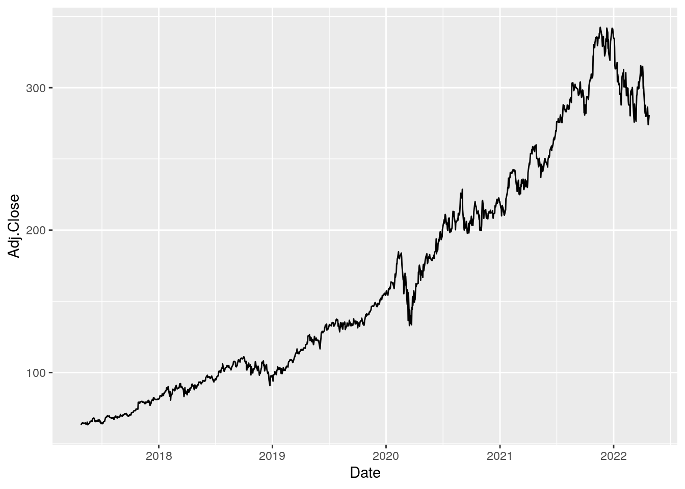
It’s a non-stationary time series, with an increasing trend in time and period of extremely high variability.
8.2.2 Preparation of the regressors and of the response variable
For the supervised problem we will use the following regressors:
- 2/7/14/21 days moving average (see @{rollingmean}) computed using past
Adj.Closevalues - 7 days rolling standard deviation computed using past
Adj.Closevalues - previous day
Volume
The following code is used for creating in the MSFT the new regressors’ columns:
MSFT$MA2 = zoo::rollmean(MSFT$Adj.Close,
                         k = 2, fill = NA, align = "right") %>%
  dplyr::lag(1)
MSFT$MA7 = zoo::rollmean(MSFT$Adj.Close,
                         k = 7, fill = NA, align = "right") %>%
  dplyr::lag(1)
MSFT$MA14 = zoo::rollmean(MSFT$Adj.Close,
                          k = 14, fill = NA, align = "right") %>%
  dplyr::lag(1)
MSFT$MA21 = zoo::rollmean(MSFT$Adj.Close,
                          k = 21, fill = NA, align = "right") %>%
  dplyr::lag(1)

MSFT$SD7 =  rollapply(data = MSFT$Adj.Close,
                      width = 7,
                      align ="right",
                      FUN = sd,
                      fill = NA) %>%
  dplyr::lag(1)

MSFT$lag1volume = dplyr::lag(MSFT$Volume,1)

head(MSFT, 25) #first top 25 rows of the df
## Date Adj.Close Close High Low Open Volume MA2 MA7
## 1 2017-04-26 63.31828 67.83 68.31 67.62 68.08 26190800 NA NA
## 2 2017-04-27 63.72900 68.27 68.38 67.58 68.15 34971000 NA NA
## 3 2017-04-28 63.90636 68.46 69.14 67.69 68.91 39548800 63.52364 NA
## 4 2017-05-01 64.79317 69.41 69.55 68.50 68.68 31954400 63.81768 NA
## 5 2017-05-02 64.69049 69.30 69.71 69.13 69.71 23906100 64.34976 NA
## 6 2017-05-03 64.48512 69.08 69.38 68.71 69.38 28928000 64.74183 NA
## 7 2017-05-04 64.23309 68.81 69.08 68.64 69.03 21749400 64.58780 NA
## 8 2017-05-05 64.41046 69.00 69.03 68.49 68.90 19128800 64.35910 64.16507
## 9 2017-05-08 64.35445 68.94 69.05 68.42 68.97 18566100 64.32178 64.32110
## 10 2017-05-09 64.44778 69.04 69.28 68.68 68.86 22858400 64.38245 64.41045
## 11 2017-05-10 64.69983 69.31 69.56 68.92 68.99 17977800 64.40112 64.48779
## 12 2017-05-11 63.90636 68.46 68.73 68.12 68.36 28789400 64.57381 64.47446
## 13 2017-05-12 63.83168 68.38 68.61 68.04 68.61 18714100 64.30309 64.36244
## 14 2017-05-15 63.87835 68.43 68.48 67.57 68.14 31530300 63.86902 64.26909
## 15 2017-05-16 65.16456 69.41 69.44 68.16 68.23 34956000 63.85502 64.21842
## 16 2017-05-17 63.35262 67.48 69.10 67.43 68.89 30548800 64.52146 64.32614
## 17 2017-05-18 63.56855 67.71 68.13 67.14 67.40 25201300 64.25859 64.18303
## 18 2017-05-19 63.54977 67.69 68.10 67.43 67.50 26961100 63.46059 64.05742
## 19 2017-05-22 64.26327 68.45 68.50 67.50 67.89 16237600 63.55916 63.89313
## 20 2017-05-23 64.47922 68.68 68.75 68.38 68.72 15425800 63.90652 63.94412
## 21 2017-05-24 64.56371 68.77 68.88 68.45 68.87 14593900 64.37124 64.03662
## 22 2017-05-25 65.36172 69.62 69.88 68.91 68.97 21854100 64.52146 64.13453
## 23 2017-05-26 65.68095 69.96 70.22 69.52 69.80 19827900 64.96272 64.16269
## 24 2017-05-30 66.10342 70.41 70.41 69.77 69.79 17072800 65.52134 64.49531
## 25 2017-05-31 65.56825 69.84 70.74 69.81 70.53 30436400 65.89218 64.85744
## MA14 MA21 SD7 lag1volume
## 1 NA NA NA NA
## 2 NA NA NA 26190800
## 3 NA NA NA 34971000
## 4 NA NA NA 39548800
## 5 NA NA NA 31954400
## 6 NA NA NA 23906100
## 7 NA NA NA 28928000
## 8 NA NA 0.5403347 21749400
## 9 NA NA 0.3925384 19128800
## 10 NA NA 0.2941575 18566100
## 11 NA NA 0.1934688 22858400
## 12 NA NA 0.1708033 17977800
## 13 NA NA 0.2460612 28789400
## 14 NA NA 0.3079325 18714100
## 15 64.19174 NA 0.3421353 31530300
## 16 64.32362 NA 0.4965557 34956000
## 17 64.29674 NA 0.6168428 30548800
## 18 64.27261 NA 0.6429121 25201300
## 19 64.18379 NA 0.5966703 26961100
## 20 64.15328 NA 0.6130147 16237600
## 21 64.15286 NA 0.6414197 15425800
## 22 64.17647 64.17267 0.6651045 14593900
## 23 64.24442 64.26998 0.7180622 21854100
## 24 64.33917 64.36293 0.8132354 19827900
## 25 64.45743 64.46755 0.8923094 17072800The following code returns the plot containing the original time series together with two rolling mean series and the rolling sd time series:
# Plot adjusted close prices + MA + SD
MSFT %>%
  ggplot() +
  geom_line(aes(Date,Adj.Close)) +
  geom_line(aes(Date,MA2,col="MA2")) +
  geom_line(aes(Date,MA21,col="MA21"),lwd=1.2) +
  geom_line(aes(Date,SD7,col="SD7"))
## Warning: Removed 2 row(s) containing missing values (geom_path).## Warning: Removed 21 row(s) containing missing values (geom_path).## Warning: Removed 7 row(s) containing missing values (geom_path).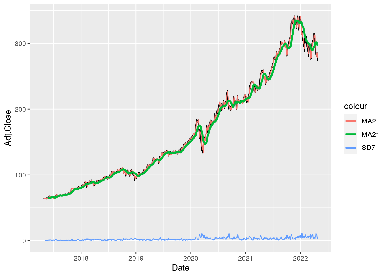
The option col="..." is not used here for setting a specific color (which will be instead chosen automatically by R) but only for creating easily a legend with the lines names (otherwise we should reshape the code and more code is needed…). The MA2 time series is very similar to the original price series, while the MA21 series is smoother (it catches the general trend but not the fine details). The SD7 has a different range of values and shows peaks during periods of high volatility.
We finally create a new column for the response variable, represented by the next day price (see the previous simple example):
MSFT$target = lead(MSFT$Adj.Close, 1)
head(MSFT)
## Date Adj.Close Close High Low Open Volume MA2 MA7 MA14 MA21
## 1 2017-04-26 63.31828 67.83 68.31 67.62 68.08 26190800 NA NA NA NA
## 2 2017-04-27 63.72900 68.27 68.38 67.58 68.15 34971000 NA NA NA NA
## 3 2017-04-28 63.90636 68.46 69.14 67.69 68.91 39548800 63.52364 NA NA NA
## 4 2017-05-01 64.79317 69.41 69.55 68.50 68.68 31954400 63.81768 NA NA NA
## 5 2017-05-02 64.69049 69.30 69.71 69.13 69.71 23906100 64.34976 NA NA NA
## 6 2017-05-03 64.48512 69.08 69.38 68.71 69.38 28928000 64.74183 NA NA NA
## SD7 lag1volume target
## 1 NA NA 63.72900
## 2 NA 26190800 63.90636
## 3 NA 34971000 64.79317
## 4 NA 39548800 64.69049
## 5 NA 31954400 64.48512
## 6 NA 23906100 64.23309We then remove all the rows containing missing values and select only the useful columns:
MSFT = MSFT %>%
  na.omit() %>%
  dplyr::select(Date, MA2, MA7, MA14, MA21, SD7, lag1volume, target)

head(MSFT)
## Date MA2 MA7 MA14 MA21 SD7 lag1volume target
## 22 2017-05-25 64.52146 64.13453 64.17647 64.17267 0.6651045 14593900 65.68095
## 23 2017-05-26 64.96272 64.16269 64.24442 64.26998 0.7180622 21854100 66.10342
## 24 2017-05-30 65.52134 64.49531 64.33917 64.36293 0.8132354 19827900 65.56825
## 25 2017-05-31 65.89218 64.85744 64.45743 64.46755 0.8923094 17072800 65.81235
## 26 2017-06-01 65.83583 65.14579 64.51946 64.50446 0.7059899 30436400 67.37083
## 27 2017-06-02 65.69030 65.36709 64.65560 64.55788 0.6209101 21603600 67.85901The following code represents graphically the correlation between the considered variables:
library(ggcorrplot)
ggcorrplot(cor(MSFT[,-1]),
           hc.order = TRUE,
           type = "lower",
           lab = TRUE, digits=4)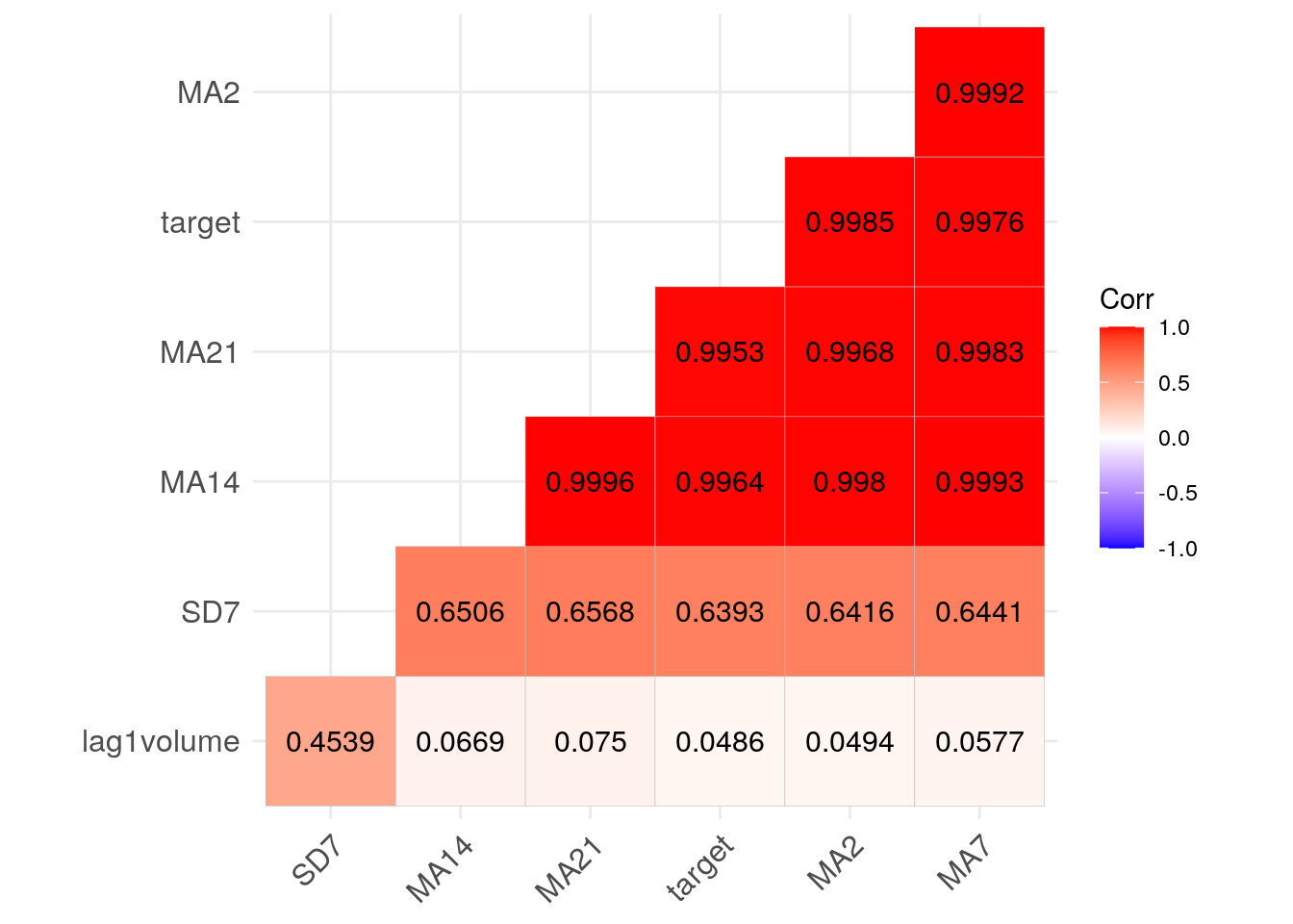
8.2.3 Training and test set
When we work with time series we want to create the training and test set without breaking the temporal sequence of the data (and the related temporal correlation). For this reason we don’t select training data randomly (as done in Section 6.1.1, but we select the observations from 2017 to the end of 2021 as training data and the remaining data for the test (i.e. for evaluating the predictive performance of the model). The row selection is done using the information about the year which can be extracted from the full date using the year function from lubridate:
MSFTtr = MSFT %>%
  filter(year(Date) < 2022)
MSFTte = MSFT %>%
  filter(year(Date) >= 2022)
With this approach the percentage of data dedicated to the training is the following:
nrow(MSFTtr)/nrow(MSFT)*100## [1] 93.77526The number of test observations is equal to 77.
8.2.4 Data normalization
By using the function normalize we normalized all the columns in the MSFT dataframe but not Date. To implement the normalization functionn by column (i.e. separately for each variable) we will use the function apply (see ?apply):
MSFTtr = data.frame(apply(MSFTtr[,-1],2,normalize))
head(MSFTtr)
## MA2 MA7 MA14 MA21 SD7 lag1volume
## 1 0.0005927972 0.0000000000 0.0000000000 0.0000000000 0.05296239 0.06904779
## 2 0.0021850423 0.0001024794 0.0002496531 0.0003594390 0.05802160 0.13898080
## 3 0.0042008004 0.0013126507 0.0005977847 0.0007027827 0.06711377 0.11946367
## 4 0.0055389817 0.0026301730 0.0010322950 0.0010892422 0.07466795 0.09292550
## 5 0.0053356564 0.0036793010 0.0012602073 0.0012255786 0.05686829 0.22164877
## 6 0.0048105012 0.0044844521 0.0017604226 0.0014229115 0.04874037 0.13656789
## target
## 1 0.006036340
## 2 0.007553825
## 3 0.005631552
## 4 0.006508324
## 5 0.012106306
## 6 0.013859796MSFTte = data.frame(apply(MSFTte[,-1],2,normalize))
head(MSFTte)## MA2 MA7 MA14 MA21 SD7 lag1volume target
## 1 1.0000000 0.9960674 1.0000000 0.9876331 0.09785490 0.0000000 1.0000000
## 2 0.9618317 1.0000000 0.9925227 0.9934102 0.06212817 0.1500012 0.7678880
## 3 0.9007791 0.9855889 0.9936001 1.0000000 0.21994156 0.2025940 0.7219434
## 4 0.7473543 0.9194452 0.9642216 0.9892257 0.66243705 0.3044882 0.7248838
## 5 0.6209897 0.8500031 0.9465012 0.9661175 0.88719009 0.2988522 0.7291106
## 6 0.6014462 0.7791910 0.9308069 0.9431301 0.89798474 0.2032250 0.7421593The second input of the apply function is the MARGIN option. It is equal to 2 if you want to compute the required function (normalize) column by column. Otherwise it can be 1 if you want to do the computation row by row. We use the data.frame in order to be sure that the final object is a data frame (and not a matrix).
8.2.5 Regression tree
We have now the data to estimate the regression tree for predicting the MSFT price, given the 6 selected regressors.
We use now the training data to estimate a regression tree by using the rpart function of the rpart package (see ?rpart). As usual we have to specify the formula, the dataset and the method (which will be set to anova for a regression tree). More information about the anova methodology can be find into this document here (page 32).
pricetree = rpart(formula = target ~.,
                  data =  MSFTtr,
                  method = "anova")
Note that some options that control the rpart algorithm are specified by means of the rpart.control function (see ?rpart.control). In particular, the cp option, set by default equal to 0.01, represents a pre-pruning step because it prevents the generation of non-significant branches (any split that does not decrease the overall lack of fit by a factor of cp is not attempted). See also the meaning of the minsplit, minbucket and maxdepth options.
It is possible to plot the estimated tree as follows:
rpart.plot(pricetree)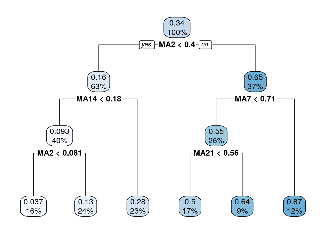
The function rpart.plot has different options about which information should be displayed. Here we use it with its default setting and each node provides the average price and the percentage of training observations in each node (with respect to the total number of training observations). Note that basically all the numbers in the plot are rounded.
It is also possible to analyze the structure of the tree by printing it:
pricetree## n= 1160
##
## node), split, n, deviance, yval
## * denotes terminal node
##
## 1) root 1160 84.7423800 0.34201040
## 2) MA2< 0.4017356 729 7.8698120 0.16016720
## 4) MA14< 0.1809473 465 1.2662160 0.09315739
## 8) MA2< 0.0809836 183 0.1166070 0.03702299 *
## 9) MA2>=0.0809836 282 0.1987565 0.12958500 *
## 5) MA14>=0.1809473 264 0.8378773 0.27819590 *
## 3) MA2>=0.4017356 431 11.9938400 0.64958280
## 6) MA7< 0.7050037 296 1.9696930 0.55132710
## 12) MA21< 0.5648444 192 0.4525512 0.50105920 *
## 13) MA21>=0.5648444 104 0.1363078 0.64412940 *
## 7) MA7>=0.7050037 135 0.9008853 0.86501730 *The most important regressor, which is located in the root node, is MA2 (so basically information referring to very few past data).
Given the grown tree we are now able to compute the predictions for the test set and to compute, as measure of performance, the mean squared error (\(MSE = \sum_{i=1}^n(y_i-\hat y_i)^2\) with \(i\) denoting the generic observation in the test set). The predictions can be obtained by using the predict function that will return the vector of predicted prices:
pricepred = predict(object = pricetree,
                    newdata = MSFTte)

head(pricepred)
## 1 2 3 4 5 6
## 0.8650173 0.8650173 0.8650173 0.8650173 0.8650173 0.8650173# MSE
mean((MSFTte$target - pricepred)^2)## [1] 0.03220142We also predict the observed test data and the corresponding predictions:
# Define first a data.frame before using ggplot
data.frame(obs = MSFTte$target, pred = pricepred) %>%
  ggplot() +
  geom_line(aes(1:nrow(MSFTte),obs, col="obs")) +
  geom_line(aes(1:nrow(MSFTte),pred, col="pred"))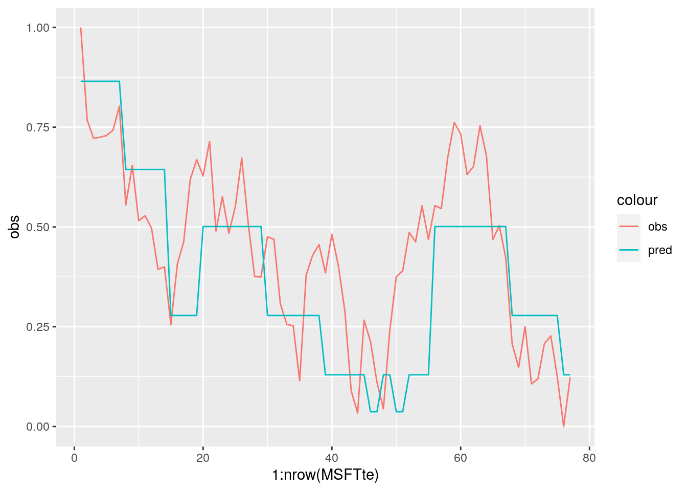
We see that the regression tree is able to get the trend of the test set but it is not doing a good job in the prediction (with many period of constant prediction). We will try to do better by using an ensemble method, like bagging, random forest or boosting.
8.3 Exercises Lab 6
8.3.1 Exercise 1
Consider the data in the file Adjcloseprices.csv: it contains the adjusted close prices for Apple (AAPL) and the values of the NASDAQ index (IXIC). There is also a column containing dates.
- Import the data and check the length of the time series.
- Plot the time series for APPL and the NASDAQ index (to do this you have first to set properly the dates).
- Knowing that AAPL price is the target variable, compute the following regressors and set properly the data frame:
- moving average of the past 2/7/14 and 21 AAPL prices
- rolling standard deviation of the past 7 and 21 AAPL prices
- the past two values of the NASDAQ index.
Include also the column for the prices to be predicted.
Consider the first 70% of the data for training and the remaining data for test. Prepare the two data frames, removing the missing values, and then normalize the data.
Implement a regression tree for predicting AAPL price using the 7 regressors defined above. Plot the estimated regression tree.
Given the above computed tree, compute the MSE and plot in the same chart predicted and observed AAPL values.