Chapter 4 Multiple Linear Regression III: Further topics

4.1 Prediction of mean response and new observations

In many ocasions, we want to create confidence intervals not only for the parameters, but also for the mean response, $E(Y_h)$, for a particular set of values of the predictors $\mathbf{X}_h=[1,x_{h1}, x_{h2},\ldots, x_{hk}]$. Since $\mathbf{\hat Y}=\mathbf{X}\boldsymbol{\hat \beta}$, the predicted value of the mean response at $\mathbf{X}_h$ is $\hat Y_h=\mathbf{X}_h\boldsymbol{\hat \beta}$, and \[\hat Y_h \sim N(\mathbf{X}_h\boldsymbol{\beta}, \sigma^2\mathbf{X}_h(\mathbf{X}^\prime \mathbf{X})^{-1} \mathbf{X}_h^\prime).\]

Sometimes we require a confidence interval for a new observation. For example, suppose that you are interested in your predicted hydrostatic measure of percent fat (given your abdominal and triceps fat and your age) and not on the average hydrostatic measure that is assigned to all people that have the same measurements and age as you. Although the point estimate for you ($\hat Y_{h(new)}$) and the average ($E[Y_h]$) will be the same, the variance of the prediction will not. In this case we are not estimating a parameter, we are predicting a random variable, and so, we need the variance of the prediction error in order to calcultate the confidence interval for the prediction: $$Var(Y_h-Y_{h(new)})=Var (Y_h) + Var(Y_{h(new)})=^2 ( 1+_h(⁾{-1} _h^ Why the covariance between $Y_h$ and $\hat Y_{h(new)}$ is zero?

To compute confidence intervals, the function predict.lm() has the argument intervalwich has the option of calculating the confidence interval for the mean or the prediction interval for a new observation.

Let’s calculate, using mod3, the predicted value and the confidence and prediction intervals for the following values of the predictors: age= 17.5, abs= 10.5 and triceps=20

#construct new data
new=data.frame(age=7.5,abs=10.5, triceps=20)
predict(mod3,newdata=new,interval="confidence")

##        fit     lwr      upr
## 1 19.67252 15.2064 24.13864

predict(mod3,newdata=new,interval="prediction")

##        fit      lwr      upr
## 1 19.67252 12.21365 27.13139

4.2 Transformations

There are many reasons to transform data as part of a regression analysis:

To achieve linearity.
To achieve homogeneity of variance, that is, constant variance about the regression equation.
To achieve normality or, at least, symmetry about the regression equation.

4.2.1 Transformations of predictors

They are generally used to linearize the relationship between the response and the predictor. After the transformation, the resduals in the new model need to be analyzed again to check if all assumptions are satisfied.

We can see it in the following example:


simu=read.table(file = "./Datasets/Transform.txt", header = TRUE)

#Model with x1
m1=lm(y~x1,data=simu)

#plot data and residuals
par(mfrow=c(1,3))
plot(simu$x1, simu$y, xlab="x1",ylab="y")
plot(m1,which=c(1,2))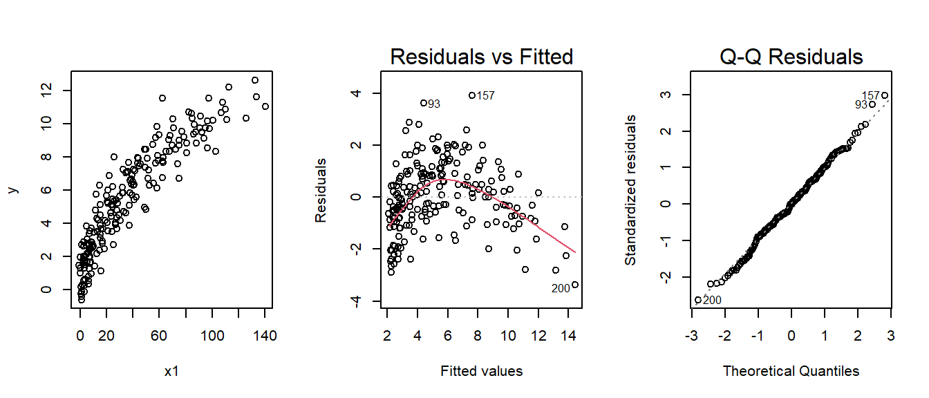

From the first and second plot we can clearly see that the relationship between x1 and y is non-linear. The pattern suggest a square root transformation.


#Model with transformed y
m2=lm(y~I(x1^0.5),data=simu)

#plot data and residuals
par(mfrow=c(1,3))
plot((simu$x1)^0.5, simu$y, xlab="x1",ylab="y")
plot(m2,which=c(1,2))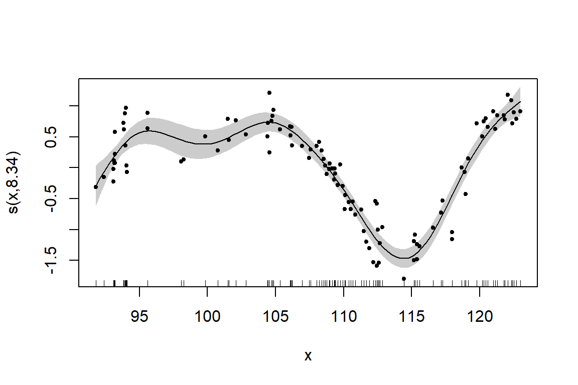

Now the plots looks fine. The identity function I() needs to be used when we whan to do arithmetic operations with variables within a formula.

Exercise 7

Find the appropriate transformation for x2 and x3 in the Transform.txt dataset and use the residual graphs to show that the transformed model is correct.

4.2.2 Transformations of response variable

Transformation of the response are commonly used to achieve normality and/or constant variance. One technique that searches computationally for the appropriate transformation of the response variable to address normality is the Box-Cox method. This method estimates a parameter $\lambda$ for the transformation (using maximum likelihood): \[ Y^*= \left \{ \begin{array}[h]{ll} \frac{Y^\lambda-1}{\lambda} & \lambda \neq 0 \\ ln \left ( Y \right ) & \lambda=0 \end{array} \right . \]


#Model y1 ~x1
simu2=read.table(file = "./Datasets/Transform2.txt", header = TRUE)
m3=lm(y1~x2,data=simu2)

#plot data and residuals
par(mfrow=c(1,3))
plot(simu2$x1, simu2$y2, xlab="x1", ylab="y")
plot(m3,which=c(1,2))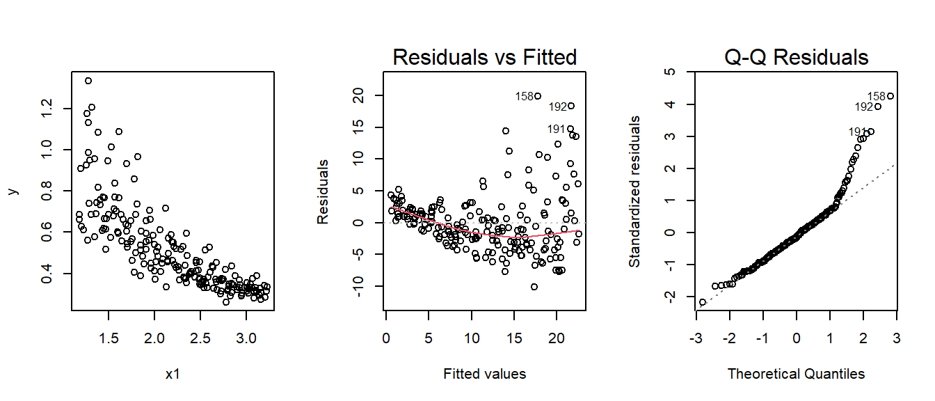

There is clearly a violation of the constant variance and normality of the residuasl. The function boxcox() of the package MASS produces a plot of the log-likelihood against the transformation parameter $\lambda$


library(MASS)
boxcox(m3)

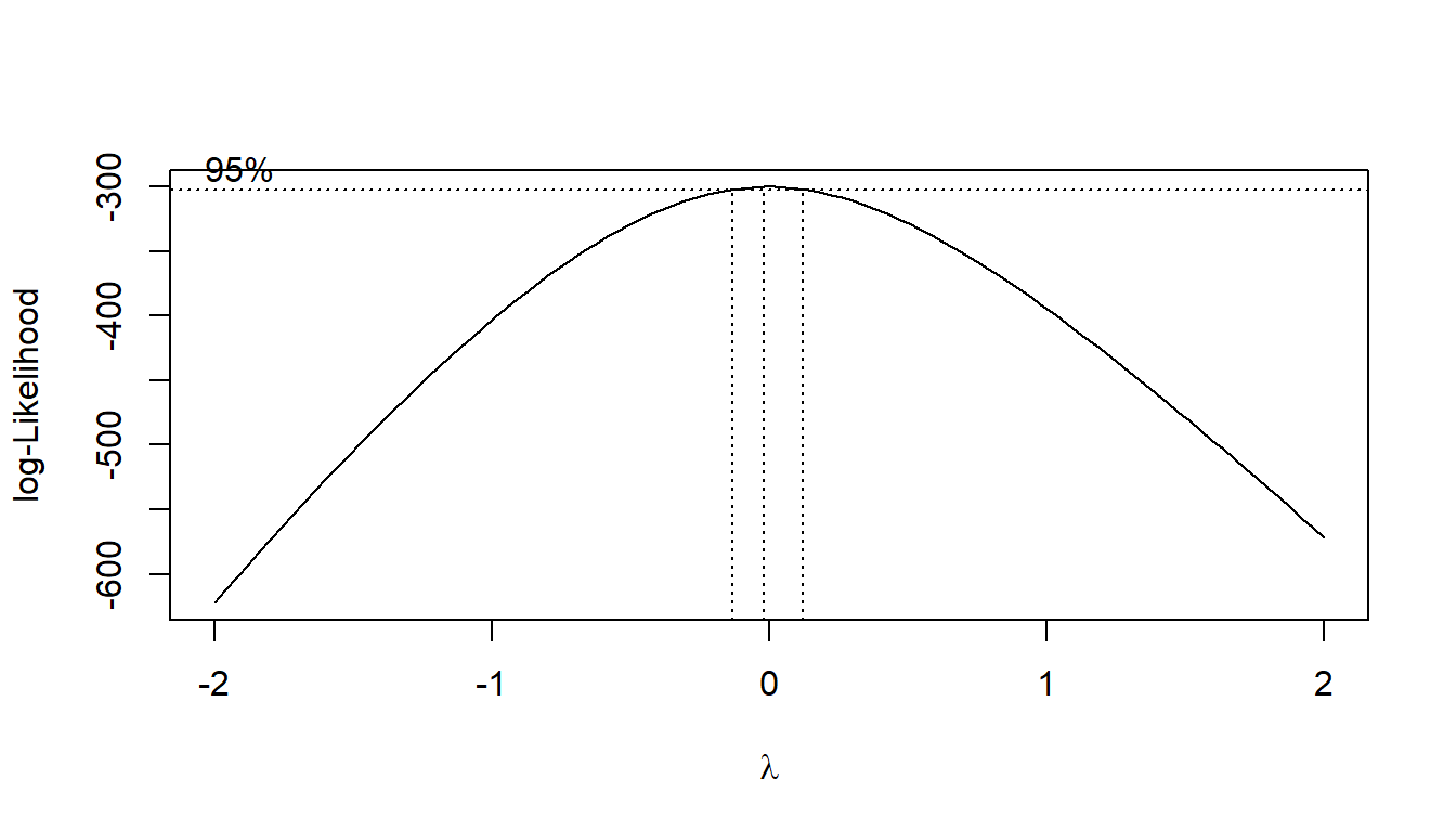The value $\lambda=-0$ is close to maximizing the likelihood (included in the 95$\%$ confidence interval. Based on these results we use the log() transformation:


#Model y2 ~x1 with  transformation

m4=lm(log(y1)~x2,data=simu2)

#plot data and residuals
par(mfrow=c(1,3))
plot(simu2$x2, log(simu2$y1), xlab="x2", ylab="y")
plot(m4,which=c(1,2))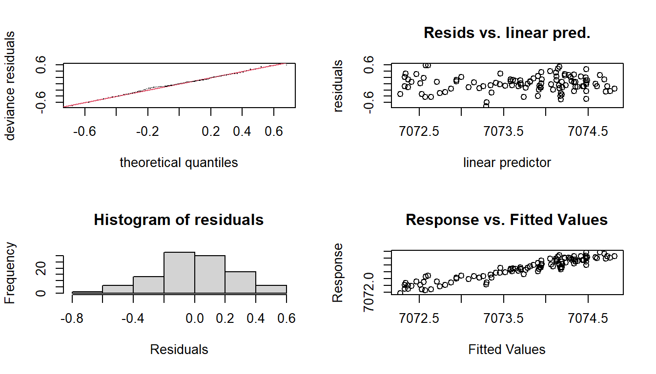

4.3 Categorical predictors

Models with factor (o categorical) variables as predictors are simply special cases of regression models by means of the use of dummy variables (in general, a dummy variable is a variable that takes only values 0 or 1). Provided that a regression model includes an intercept, and our categorical variable has $k$ different levels, one needs to greate $k-1$ dummy variables regression models.

We are going to use the dataset apartments.txt to show how to work with categorical variables. This dataset has information on the price of 218 flats and different characteristics that might have an impact on the price: area, number of rooms and bathrooms, etc. One of the variables in the dataset is called elevator and it takes value 1 if the apartment is accesible by elevator, and 0 if it is not.

If a variable is to be treated as categorical, the first thing we need to do is to define it as a factor in R.


apartments=read.table("./Datasets/apartments.txt")
#Check that the variable is define as numeric
summary(apartments$elevator)
##    Min. 1st Qu.  Median    Mean 3rd Qu.    Max. 
##  0.0000  1.0000  1.0000  0.7982  1.0000  1.0000

#Define the variable as factor and check it
apartments$elevator=factor(apartments$elevator)
summary(apartments$elevator)
##   0   1 
##  44 174

We want to fit the model that uses elevator as predictor:

\[Y_i=\beta_0+\beta_1 \, elevator_i+\varepsilon_i.\] For flats with elevator access: \[E[Y_i]=\beta_0+\beta_1,\] and for the ones without access: \[E[Y_i]=\beta_0.\] Then, the interpretation of the estimated parameters will be: $\hat \beta_0$ is the average price of flats without elevator access and $\hat \beta_1$ is the the increase or decrease in mean price in comparison with flats without elevator access.


#Fit a model with the variable `elevator`
flats1=lm(totalprice~elevator, data=apartments)
summary(flats1)
## 
## Call:
## lm(formula = totalprice ~ elevator, data = apartments)
## 
## Residuals:
##    Min     1Q Median     3Q    Max 
## -98506 -41006 -13006  35423 261494 
## 
## Coefficients:
##             Estimate Std. Error t value Pr(>|t|)    
## (Intercept)   210492       9001  23.385  < 2e-16 ***
## elevator1      88014      10075   8.736 6.76e-16 ***
## ---
## Signif. codes:  0 '***' 0.001 '**' 0.01 '*' 0.05 '.' 0.1 ' ' 1
## 
## Residual standard error: 59710 on 216 degrees of freedom
## Multiple R-squared:  0.2611, Adjusted R-squared:  0.2576 
## F-statistic: 76.31 on 1 and 216 DF,  p-value: 6.764e-16

The test for $\beta_1=0$ is testing if the mean increase in price (88014 euros) is significant (it is).

Finally, note that including a binary variable that is 0 for those with elevator access and 1 for the ones without access would be redundant, it would create three parameters to describe two means. If we include both dummies the matrix of covariates $\mathbf{X}$ would be: \[X=\left [ \begin{array}[h]{lll} 1 & 1 &0\\ 1 &1 &0 \\ \vdots & \vdots & \vdots \\ 1 &1 &0 \\ 1 & 0&1 \\ 1 & 0&1 \\ \vdots & \vdots & \vdots \\ 1 & 0&1 \\ \end{array}\right ]\]

We can inmediatly see that we can obtain the third column by substracting the second from the first, therefore we would have exact collinearity and the model could not be fitted.

But, what happens if there are more than two categories?. To illustrate this case we look at the variable heating which has 4 levels:

1A: no-heating
3A: low-standard private heating
3B: high-standard private heating
4A: central heating

R has already recognized this variable as categorical since the levels are especified as characters, but we will define it as a factor

#Check that the variable is defined as a factor
summary(apartments$heating)
##    Length     Class      Mode 
##       218 character character
apartments$heating=factor(apartments$heating)

Now the model would be: \[Y_i=\beta_0+\beta_1 3A_i+\beta_2 3B_i+ \beta_3 4A_i\varepsilon_i,\] where $3A$ is a dummy variable that takes value 1 if the apartment has low-standard private heating and 0 if it doesn’t (3B and 4A are defined similarly). As before, there is no need to define a dummy variable for 1A since it would be redundant. In principle we can choose the level of the categorical variable that is associated with $\beta_0$. By default, R takes the one with the lowest numerical value or, if the levels are characters, the first one in alphabetical order.

#Fit a model with `heating` as predictor
flats2=lm(totalprice~heating,data=apartments)
summary(flats2)
## 
## Call:
## lm(formula = totalprice ~ heating, data = apartments)
## 
## Residuals:
##     Min      1Q  Median      3Q     Max 
## -109023  -48963  -13543   40650  208207 
## 
## Coefficients:
##             Estimate Std. Error t value Pr(>|t|)    
## (Intercept)   204625      22680   9.022  < 2e-16 ***
## heating3A      65168      23281   2.799  0.00559 ** 
## heating3B     148275      30428   4.873 2.14e-06 ***
## heating4A     105895      24394   4.341 2.19e-05 ***
## ---
## Signif. codes:  0 '***' 0.001 '**' 0.01 '*' 0.05 '.' 0.1 ' ' 1
## 
## Residual standard error: 64150 on 214 degrees of freedom
## Multiple R-squared:  0.155,  Adjusted R-squared:  0.1431 
## F-statistic: 13.08 on 3 and 214 DF,  p-value: 7.067e-08

In this case, each estimated parameter shows the increse (since all a positive) in mean price of the apartments compared with the ones with no heating, and the intercept (204625 euros) is the mean price for a flat with no heating. If we drop the intercept:


flats2.2=lm(totalprice~heating-1,data=apartments)
summary(flats2.2)
## 
## Call:
## lm(formula = totalprice ~ heating - 1, data = apartments)
## 
## Residuals:
##     Min      1Q  Median      3Q     Max 
## -109023  -48963  -13543   40650  208207 
## 
## Coefficients:
##           Estimate Std. Error t value Pr(>|t|)    
## heating1A   204625      22680   9.022   <2e-16 ***
## heating3A   269793       5255  51.339   <2e-16 ***
## heating3B   352900      20285  17.397   <2e-16 ***
## heating4A   310520       8982  34.570   <2e-16 ***
## ---
## Signif. codes:  0 '***' 0.001 '**' 0.01 '*' 0.05 '.' 0.1 ' ' 1
## 
## Residual standard error: 64150 on 214 degrees of freedom
## Multiple R-squared:  0.9517, Adjusted R-squared:  0.9508 
## F-statistic:  1054 on 4 and 214 DF,  p-value: < 2.2e-16

Now, the flats with no heating appear. What is being tested now?

Also, if there are no other covariates, the estimated coefficients for this model are exactly the empirical means of the groups. We can use the dplyr package to check this and grab the mean for each group:

#Calculate means for each group
library(dplyr)
summarise(group_by(apartments, heating), mn = mean(totalprice))
## # A tibble: 4 × 2
##   heating      mn
##   <fct>     <dbl>
## 1 1A      204625 
## 2 3A      269793.
## 3 3B      352900 
## 4 4A      310520.

If you look back to model flat2, each mean is obtained as the sum of the intercept in that model plus each coefficients, for example, the mean for flats with low quality individual heating (3A) is 269793=204625+65168.

Often your lowest alphanumeric level isn’t the level that you’re most interested in as a reference group. There’s an easy fix for that with factor variables; use the reorder() function in the DescTools package. Let’s create a variable heating2 that has cental heating (4A) as the reference level:

library(DescTools)
#reorder the coefficients and fit again the model
heating2=  relevel(factor(apartments$heating), ref="4A")
summary(lm(totalprice ~ heating2, data = apartments))$coef
##               Estimate Std. Error   t value     Pr(>|t|)
## (Intercept)  310519.61    8982.46 34.569552 1.551155e-89
## heating21A  -105894.61   24393.62 -4.341078 2.187041e-05
## heating23A   -40726.64   10406.80 -3.913465 1.222487e-04
## heating23B    42380.39   22185.04  1.910314 5.742963e-02

you can check the difference by using the contrast() funcion:

#Check how the dummy variables are created
contrasts(factor(apartments$heating))
##    3A 3B 4A
## 1A  0  0  0
## 3A  1  0  0
## 3B  0  1  0
## 4A  0  0  1
contrasts(heating2)
##    1A 3A 3B
## 4A  0  0  0
## 1A  1  0  0
## 3A  0  1  0
## 3B  0  0  1

The rows are the levels of the variable and the columns are the dummy variables.

Summary on categorical variables

If we treat a variable as a factor, R includes an intercept and omits the alphabetically (or numerically) first level of the factor.
- The intercept is the estimated mean for the reference level.
- The intercept t-test tests for whether or not the mean for the reference level is 0.
- All other t-tests are for comparisons of the other levels versus the reference level.
- Other group means are obtained the intercept plus their coefficient.
If we omit an intercept, then, it includes terms for all levels of the factor.
- Group means are now the coefficients.
- Tests are t-tests of whether the groups’ means are different than zero.
If we want comparisons between two levels, neither of which is the reference level, we could refit the model with one of them as the reference level.

In general, in a model we will have both numerical and cathegorical variables. We are going to illustrate how to interpret the results of the model when a continuos ($\mathbf{x}$) and a categorical variable ($\mathbf{D}$) are included (and their interaction). For simplicity we will assume that the categorical variable only has two levels. Our model would be: \[\mathbf{Y}=\beta_0+\beta_1\mathbf{x} +\beta_2 \mathbf{D} +\beta_3 \mathbf{x} \mathbf{D}+\boldsymbol{\varepsilon} \] Since $\mathbf{D}$ is coded with 1 or 0, we have in fact two lines:

If $\mathbf{D}=0: \mathbf{Y}=\beta_0+\beta_1\mathbf{x}+\boldsymbol{\varepsilon}$
If $\mathbf{D}=1$: $\mathbf{Y}=\beta_0+\beta_2+(\beta_1+\beta_3)\mathbf{x}+\boldsymbol{\varepsilon}$

This type of model requires to answer the questions:

Are both lines the same?
Are the slopes the same?
Are the intercepts the same?

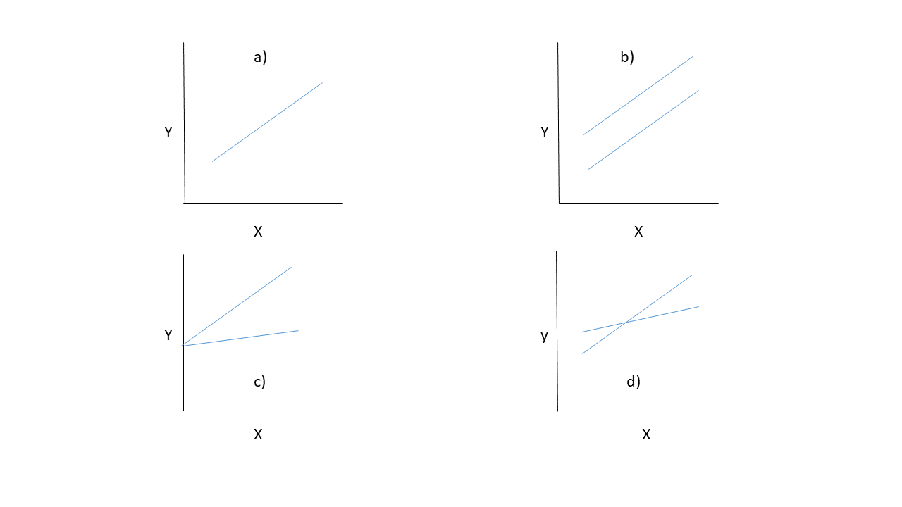
Which plot correspond to the answer of the previous questions? Which null hypothesis must be tested in each case?

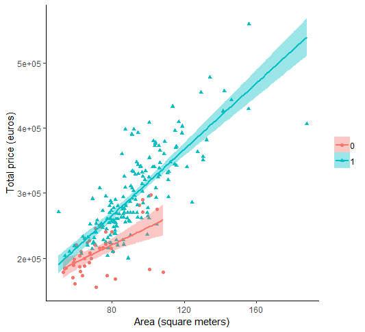
For example in the apartments dataset suppose that we include in the model the variables elevator and area (which measures the size of the apartment in $m^2$):

#Fit the model with both variables and their interaction
modTotal=lm(totalprice~area+elevator+area:elevator,data=apartments)
summary(modTotal)
## 
## Call:
## lm(formula = totalprice ~ area + elevator + area:elevator, data = apartments)
## 
## Residuals:
##     Min      1Q  Median      3Q     Max 
## -133610  -22216   -2423   20276  113159 
## 
## Coefficients:
##                Estimate Std. Error t value Pr(>|t|)    
## (Intercept)    113114.0    28985.0   3.902 0.000128 ***
## area             1343.7      392.2   3.426 0.000735 ***
## elevator1      -50871.7    31990.6  -1.590 0.113264    
## area:elevator1   1202.0      417.4   2.880 0.004380 ** 
## ---
## Signif. codes:  0 '***' 0.001 '**' 0.01 '*' 0.05 '.' 0.1 ' ' 1
## 
## Residual standard error: 37610 on 214 degrees of freedom
## Multiple R-squared:  0.7096, Adjusted R-squared:  0.7055 
## F-statistic: 174.3 on 3 and 214 DF,  p-value: < 2.2e-16

When there is an interaction present in the model, the interpretation of the parameters should be done with care (and in general, they should not be interpreted separately):

$\hat \beta_0$ is the mean price of a flat without elevator when area=0.
$\hat \beta_1$ is the change in mean price when the apartment increse in size in $1m^2$ for flats without elevator.
$\hat \beta_2$ is the change in mean price between apartment with and without elevator (for apartments of the area=0).
$\hat \beta_3$ is the extra change in mean price when the apartment increses in size in $1m^2$ between apartments with and without elevator.

If we want to answer each of the previous questions, we need to carry out different hypothesis test:

Are both lines the same?: $H_0 : \beta_2=\beta_3=0$

Since we want to test both parameters simultaneously we need to use the Analysis of Variance:

#Fit the model without the variable `elevator`
modarea=lm(totalprice~area,data=apartments)
#Use anova table to compare models
anova(modarea,modTotal)
## Analysis of Variance Table
## 
## Model 1: totalprice ~ area
## Model 2: totalprice ~ area + elevator + area:elevator
##   Res.Df        RSS Df Sum of Sq      F    Pr(>F)    
## 1    216 3.5970e+11                                  
## 2    214 3.0267e+11  2 5.704e+10 20.165 9.478e-09 ***
## ---
## Signif. codes:  0 '***' 0.001 '**' 0.01 '*' 0.05 '.' 0.1 ' ' 1

Therefore, at least $\beta_2$ or $\beta_3$ (or both) are different from zero, and the lines are not the same

Are the slopes the same?: $H_0 :\beta_3=0$

In this case, since the argument is a single model, the anova table adds each term sequentially. Then, we only need to check the last line of the table:


anova(modTotal)
## Analysis of Variance Table
## 
## Response: totalprice
##                Df     Sum Sq    Mean Sq  F value    Pr(>F)    
## area            1 6.8239e+11 6.8239e+11 482.4846 < 2.2e-16 ***
## elevator        1 4.5308e+10 4.5308e+10  32.0352  4.83e-08 ***
## area:elevator   1 1.1732e+10 1.1732e+10   8.2949   0.00438 ** 
## Residuals     214 3.0267e+11 1.4143e+09                       
## ---
## Signif. codes:  0 '***' 0.001 '**' 0.01 '*' 0.05 '.' 0.1 ' ' 1

Based on the p-value, 0.00438, we conclude that the slopes are different.

Are the intercepts equal?: $H_0 : \beta_2=0$

What we are testing is whether the price with or withour elevator start at the same value:

#fit a model without `elevator`variable, but with the interaction
modInter=lm(totalprice~area+area:elevator,data=apartments)
anova(modInter,modTotal)
## Analysis of Variance Table
## 
## Model 1: totalprice ~ area + area:elevator
## Model 2: totalprice ~ area + elevator + area:elevator
##   Res.Df        RSS Df  Sum of Sq      F Pr(>F)
## 1    215 3.0624e+11                            
## 2    214 3.0267e+11  1 3576497188 2.5288 0.1133

In this case we do not reject the null hypothesis. Therefore the final model is:

#Final model
summary(modInter)
## 
## Call:
## lm(formula = totalprice ~ area + area:elevator, data = apartments)
## 
## Residuals:
##     Min      1Q  Median      3Q     Max 
## -125093  -21762   -2201   18117  112252 
## 
## Coefficients:
##                Estimate Std. Error t value Pr(>|t|)    
## (Intercept)    71352.08   12309.18   5.797 2.39e-08 ***
## area            1897.94     180.59  10.510  < 2e-16 ***
## area:elevator1   553.99      90.42   6.127 4.23e-09 ***
## ---
## Signif. codes:  0 '***' 0.001 '**' 0.01 '*' 0.05 '.' 0.1 ' ' 1
## 
## Residual standard error: 37740 on 215 degrees of freedom
## Multiple R-squared:  0.7061, Adjusted R-squared:  0.7034 
## F-statistic: 258.3 on 2 and 215 DF,  p-value: < 2.2e-16

with $R^2_a=0.7034$

Exercise 8

Repeat the analysis using the variables area and heating and plot the estimated lines

4.4 Multicollinearity

Ridge regression is a technique for analyzing multiple regression data that suffer from multicollinearity. When multicollinearity occurs, least squares estimates are unbiased, but their variances are large, and they may be far from the true value.

There are several ways to detect multicolinearity:

Condition Number

This measure is based on the eigenvalues of the model variable matrix $\mathbf{X}$ (without the columns of 1’s). If variables are correlated, this matrix will be close to be rank defficient, and so it will have eigenvalues close to zero. The condition number is defined as: \[ C.N. = \sqrt{\frac{\lambda_{max}}{\lambda_{min}}},\] where $\lambda_{max}$ and $\lambda_{min}$ are the maximum and minimun eigenvalue of $\mathbf{X^\prime\mathbf{X}}$.

If the CN is between 20 and 30, this is an indicator for a high linear multicollinearity, if it is greater than 30 it is severe. In R the function kappa() (whose argument is the matrix $\mathbf{X}$ without the columns of 1’s) return the condition number.

Variance Inflation Factor

This method is based on regressing each predictor $\mathbf{X}_j$ on the others. If the one predictor is linearly related to others, the $R^2_j$ obtained from that regression will be close to 1. This fact is used to define the Variance Inflation Factor (VIF): \[ VIF_j=\frac{1}{1-R^2_j}.\] The larger $R^2_j$ is, the large the VIF is. The $VIF_j$ for a predictor $\mathbf{X}_j$ can be interpreted as the factor ($\sqrt{VIF_j}$) by wich the standard error of $\hat \beta_j$ is incresed due to multicollinearity.

If $VIF \geq 10$, this indicates the presence of multicollinearity between explanatory variables. In R the function vif() (whose argument is a linear model) in the package car calculates the VIF.

We mentioned in 2.6 that one way to proceed when there is multicollinearity is to eliminate the redundant variables. However, it might be of interest to keep them in the model (for scientific of practical purposes). In that case we can fit the model using Ridge Regression.

Ridge Regression

It as introduced by Hoerl and Kennard (1970), and is an alternative method to the standard method of ordinary least squares in the presence of multicollinearity. The method implies adding a small positive constant ($\lambda$) to the main diagonal elements of the matrix $\mathbf{X}^\prime \mathbf{X}$. This positive value, known as the ridge parameter, decodes the links between the explanatory variables: \[ \boldsymbol{\hat \beta}_{ridge}=\left ( \mathbf{X}^\prime\mathbf{X}+\lambda\mathbf{I}\right )^{-1}\mathbf{X}^\prime \mathbf{Y}\] When introducing the ridge parameter $\lambda$, the variability of estimated parameters is reduced. Although the ordinary ridge regression method is biased, it produces a mean square error, $MSE=\left ( bias \left (\mathbf{\hat \beta} \right )\right )^2+Var \left (\mathbf{\hat \beta}\right )$ lower than the mean square error obtained with OLS method.

The ridge estimator $\boldsymbol{\hat \beta}_{ridge}$ is the solution of the following penalized least squares problem:

\[(\mathbf{Y}-\mathbf{X}\boldsymbol{\beta})^\prime (\mathbf{Y}-\mathbf{X}\boldsymbol{\beta})+\lambda \boldsymbol{\beta}^\prime \boldsymbol{\beta}.\] The effect of the penalty is to reduce the size of the redundant coefficients.

Exercise 9

1.Calculate $bias \left (\mathbf{\hat \beta} \right )$ 2. Show that $Var(\mathbf{\hat \beta_{OLS}})\leq Var(\mathbf{\hat \beta_{ridge}})$

4.5 Case study application

Now we will use ridge regression to predict bodyfat using all predictors available:

To do so we use the function glmnet() of the package with the same name. This function will give many values to $\lambda$ and will return the estimated coefficients using ridge regression

library(glmnet)
#Calculate the regression matrix without the intercept
X=model.matrix(hwfat ~.-1,data=bodyfat)
#the function `glmnet` will chose a range of values of the ridge parameter
#We need to specify alpha=0
fit.ridge=glmnet(X,bodyfat$hwfat,alpha=0)
#Plot estimated coefficients for different values of the ridge parameter
plot(fit.ridge,xvar="lambda",label=TRUE)
legend(6,-0.2, c("age", "ht", "wt", "abs","triceps","subscap"),lty=1:6,col=1:6)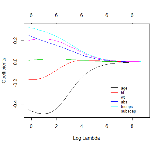

It is known that the ridge penalty shrinks the coefficients of correlated predictors towards each other, we can see how wt and ht get closer and also triceps abs and subscaps. The ridge regression will penalize the coefficients, such that, those who are the least efficient in your estimation will shrink the fastest.

What is left is to find the optimal value of $\lambda$, via cross-validation \[CV(\hat \lambda)= arg \; min \sum_{i=1}^n(Y_i-\mathbf{x}_i\hat \beta_{-i,\lambda})^2\]

#Calculate optimal ridge parameter via cross-validation
#Plot mean squared error versus ridge parameter (in the log scale)
cv.out = cv.glmnet(X, bodyfat$hwfat, alpha = 0)  #alpha=0 means Ridge Regression
plot(cv.out)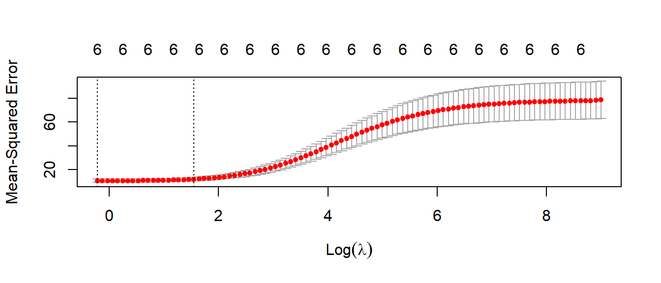

The lowest point in the curve indicates the optimal lambda: the log value of lambda that minimised the error in cross-validation. We can extract this values as:

#Getting optimal value for lambda
opt_lambda <- cv.out$lambda.min
opt_lambda
## [1] 0.8064512

#Fitting the model for that value of the ridge parameter
predict(fit.ridge, type = "coefficients", s = opt_lambda)
## 7 x 1 sparse Matrix of class "dgCMatrix"
##                      s1
## (Intercept) 19.02121047
## age         -0.45379807
## ht          -0.16474383
## wt           0.01479322
## abs          0.25139291
## triceps      0.32756185
## subscap      0.20237207

Exercise 10

Calculate the FIV for the dataset bodyfat using the function available in r and programing the code yourself
Calculate the value of $R^2$ and $R^2_a$ for model fit.ridge and compare them with the results of modall (modall <- lm(hwfat ~., data = bodyfat))

4.6 Further exercises for chapters 1 to 3

Exercise 11

Consider the following model for a random signal: \[s_i=\beta_1+\beta_2cos(\omega_i+\phi)+\varepsilon_i\quad \varepsilon_i\sim N(0,\sigma^2)\quad i=1,\ldots, 100\] The aim of this exercise is to check the distribution of the estimates of $\beta_1$ and $\beta_2$. Calculate the estimates of these parameters by simulation. To do so, give use the following values:

$\beta_1=3$
$\beta_2=3$
$\omega=(1:100)/10$
$\phi=50$
$\sigma=1$

Simulate 1000 runs of $s$ and estimate $\beta_1$ and $\beta_2$. The aim of the exercise is to show how you can check numerically one of the properties of the least squares estimates: unbiasedness. Use a histogram or any other tool to show the distribution of the estimates. How can you prove that the estimates are unbiased?. What happens if you increse the value of $\sigma$?.

Exercise 12

Use the dataset savings in the package faraway to predict savings rate (personal saving divided by disposable income) as a function of different economic variables. Once you fit the data, check if the residuals satisfy the assumptions of the linear regression model. If not, take the necessary steps to solve the problem.

Exercise 13

The Ministry of Equality has collected data in order to find a model that relates the salary to the years of education and the gender of the worker. The model obtained is: \[\widehat salary = 9.5-4.1gender+0.8education+0.2*gender:education \] where salary (annual) is expressed in thousand of euros, education in years,a nd gender takes value 0 for males and 1 for females.

What is the expected sallary of a man with 17 years of education?
What is the expected difference in salary between males a females with 12 years of education?
How many more years of education needs a woman to have the same salary as a man that has studied 15 years?

Exercise 14

The dataset insurance.csv contains data of insurance premiums paid by people in USA depending on their personal characteristics:

age: age of the policy holder
sex: male/female
bmi: body mass index
smoker: yesy/no
children: number of children
region: region where he/she lives
changres: (anual cost in dolars, of the insurance (response variable)

With this dataset:

Find the model that gives the best prediction (take into account that interactions between variables may be present)
What is the profile of the people that pay more (or less) for their insurance?. If you have to use this model help the insurance company to sell more policies, what would yo recommend?

4.7 References

References

Hoerl, A. E., and R. Kennard. 1970. “Ridge Regression: Biased Estimation for Nonorthogonal Problems.” Technometrics 12: 55–67.