Chapter 2 Multiple Linear Regression I:

Linear regression, although a basic tool in statistical modeling, is one of the most widely used techniques. As a simple illustration, consider de following figure in which we represent the reslationship between \(x=\)proverty index (the percentage of the state’s population living in households with incomes below the federally defined poverty level) and \(y=\)birth rate per 1000 females 15 to 17 years old in the U.S.

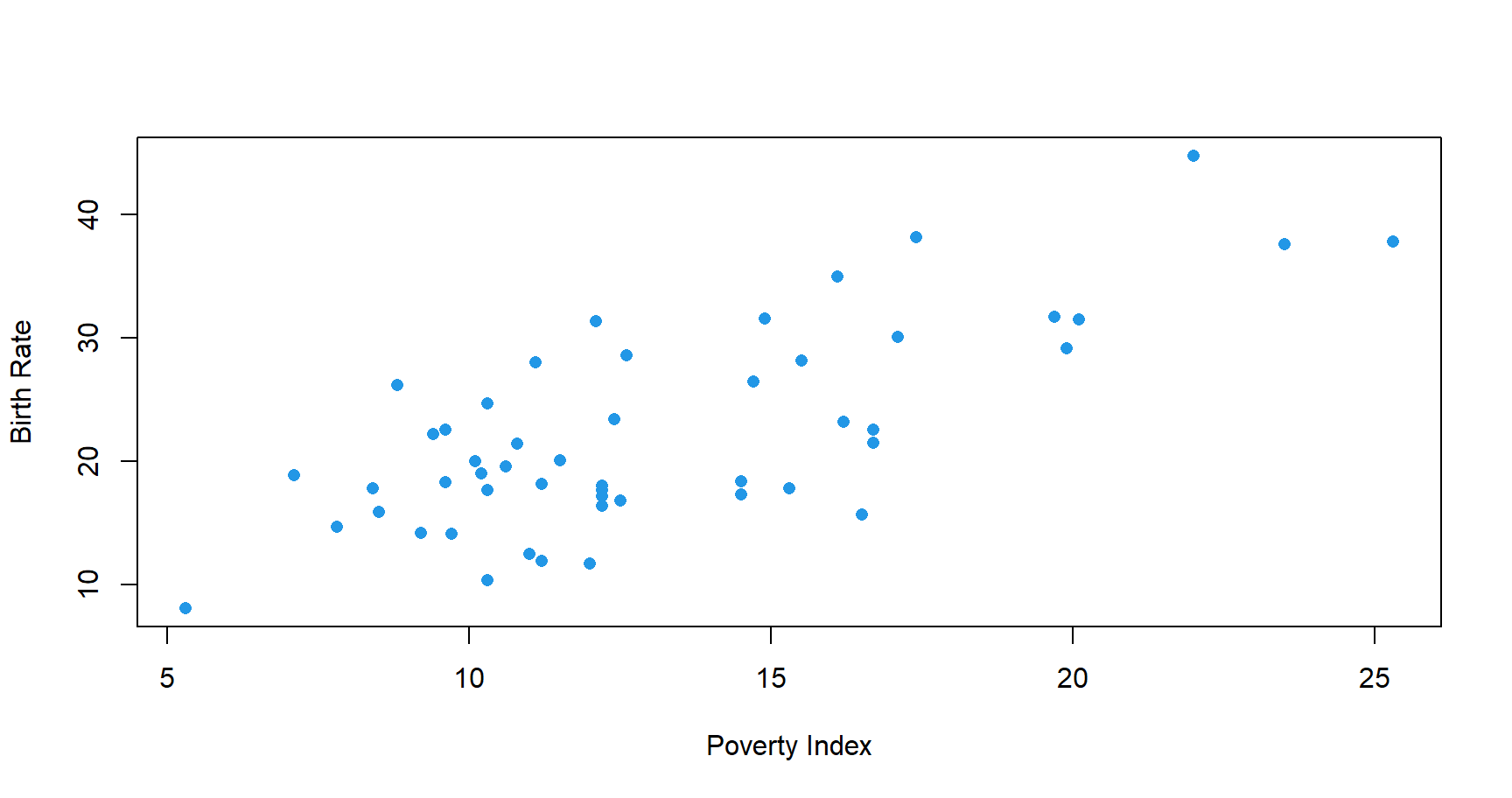
Although no simple curve will pass exactly through all the points, there is a strong indication that the points lie scattered randomly around a straight line. Therefore, it is reasonable to assume that the mean birth rate Y is related to poverty by the following straight-line relationship: \[E[Y|x]=\beta_0+\beta_1x.\] While the mean of \(Y\) is a linear function of \(x\), the actual observed values of \(Y\) do not fall on that line. The appropriate way to represent the relationship is to assume that the expected value of \(Y\) is a linear function of \(x\), but, for a fixed value of \(x\) the actual value of Y is determined by the mean value function (the linear model) plus a random error term, \[Y=\beta_0+\beta_1x+\varepsilon,\] where \(\varepsilon\) is the error term.

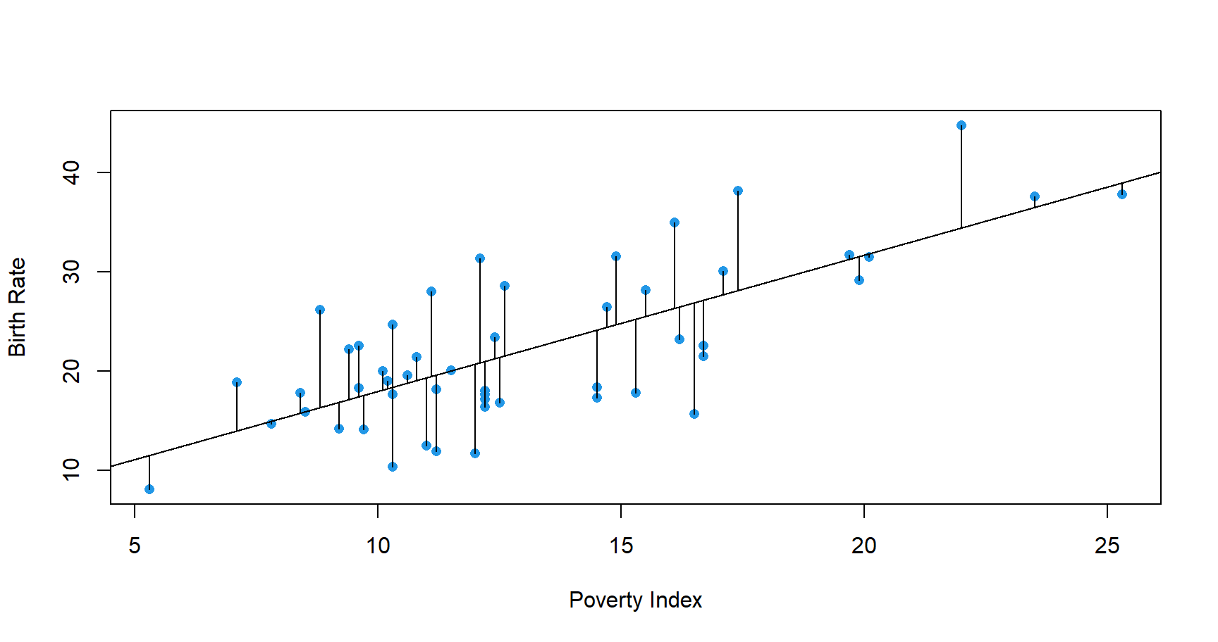We will call this model the simple linear regression model, because it has only one independent variable (regressor or covariate). However, most applications of regression analysis involve situations in which there are more than one regressor variable. A regression model that contains more than one regressor variable is called a multiple linear regression model.

2.1 Case Study: Bobyfat

Hydrostatic weighing is a type of body composition determination, meaning it measures body fat and lean mass. Using Archimedes Principle of Displacement, hydrostatic weighting measures one’s total body density.

The Archimedes Principle states that the buoyant force placed on a submerged object (in this case, you), is equal to the weight of the fluid displaced by the object. Using this principle, the hydrostatic weighing method is believed to determine the percentage of body fat in an individual’s body. This is because both the density of fat mass and fat-free mass are constant. On the other end of the spectrum, lean tissues such as muscle and bone are denser than water. With fat being less dense than water and muscle and bone being denser than water, a person who carries more body fat will be lighter underwater. A person with more muscle will weight more underwater and be less buoyant.

Hydrostatic weighing is considered the gold standard for determining body fat. However it is an expensive method, and so it, is of great interest to see whether hydrostatic fat can be predicted using different body measurements.

We will use a data set bodyfat.txt collected by Dr. Alan Utter, Department of Health Leisure and Exercise Science, Appalachian State University. It consists of hydrostatic measure of percent fat and 6 other variables measured on 78 high school wrestlers:

age: Age in years
height: Height in inches
wt: Weight in pounds
abs: Abdominal fat
triceps: Triceps fat
subscap: Subscapular fat
hwfat: Hydrostatic measure of percent fat

Table 2.1: First 10 rows of the `bodyfat` dataset.
age	ht	wt	abs	triceps	subscap	hwfat
18	65.75	133.6	8	6	10.5	10.71
15	65.50	129.0	10	8	9.0	8.53
17	64.00	120.8	6	6	8.0	6.78
17	72.00	145.0	11	10	10.0	9.32
17	69.50	299.2	54	42	37.0	41.89
14	66.00	190.6	40	25	26.0	34.03
14	63.00	108.8	6	8	7.0	7.47
17	67.25	132.6	11	7	8.0	6.08
15	69.75	148.4	9	6	8.0	7.59
14	70.50	175.4	19	13	11.5	13.08

Along this chapter we will try to answer the following questions:

Can we predict effectively the Hydrostatic measure of percent fat?
What is the effect of the different variables in such prediction?

2.2 Model formulation

Multiple linear regression is similar to the simple linear regression case in the sense that we have a response variable, \(Y\), an intercept \(\beta_0\) and an error term \(\varepsilon\), but now we have more than one covariate: \[ \begin{aligned} Y_1 &= \beta_0 +\beta_1 x_{11} +\beta_2 x_{12}+\ldots \beta_k x_{1k}+\varepsilon_1\\ Y_2 &= \beta_0 +\beta_1 x_{21} +\beta_2 x_{12}+\ldots \beta_k x_{2k}+\varepsilon_2\\ &\vdots \\ Y_n &= \beta_0 +\beta_1 x_{n1} +\beta_2 x_{n2}+\ldots \beta_k x_{nk}+\varepsilon_n\\ \end{aligned} \]

2.2.1 Matrix formulation of the model

The model above is tipically expressed in a more compact form:

\[\mathbf{Y}=\mathbf{X}\boldsymbol{\beta }+\boldsymbol{\varepsilon} \] where

\[\begin{align} \mathbf{Y}=\left [ \begin{array}[h]{c} y_1\\ y_2\\ \vdots \\ y_n \end{array} \right ]\quad \mathbf{X}=\left [ \begin{array}[h]{cccc} 1&x_{11}&\ldots&x_{1k}\\ 1&x_{21}&\ldots&x_{2k}\\ \vdots &\ddots&\vdots\\ 1&x_{n1}&\ldots&x_{nk} \end{array} \right ]\quad \boldsymbol{\beta}=\left [ \begin{array}[h]{c} \beta_0\\ \beta_1\\ \vdots \\ \beta_k \end{array} \right ] \quad \boldsymbol{\varepsilon}=\left [ \begin{array}[h]{c} \varepsilon_1\\ \varepsilon_2\\ \vdots \\ \varepsilon_n \end{array} \right ] \tag{2.1} \end{align}\]

Each column of \(\mathbf{X}\) contains values of a particular covariate, and their are assumed to be known, \(\boldsymbol{\beta}\) is the vector of unknown parameters (constants) to be estimated from the model, and \(\mathbf{Y}\) and \(\boldsymbol{\varepsilon}\) are random vectors whose elements are random variables.

2.3 Model assumptions

The regression model is formulated under certain assumptions that we need to be aware off, since they need to be satisfied in order to make use of the model:

Linearity: The mean of the response, is a linear function of the predictors, \[E[\mathbf{Y}|\mathbf{X}_1=x_1,\ldots,\mathbf{X}_k=x_k ]=\beta_0+\beta_1 x_1+\ldots +\beta_k x_k\].
Independence: The errors, \(\varepsilon_i\), are independent, \[Cov[\varepsilon_i,\varepsilon_j]=0\quad i\neq j\].
Homocedasticity: The variance of the errors, \(\varepsilon_i\), at each value of the predictor, \(x_i\), is constant. \[Var[\varepsilon_i|\mathbf{X}_1=x_1,\ldots,\mathbf{X}_k=x_k ]=\sigma^2\]
Normality: The errors, \(\varepsilon_i\), are Normally distributed \[\varepsilon_i \sim N(0,\sigma^2)\]

In summary: \[ \boldsymbol{\varepsilon}\sim N(\mathbf{0}, \mathbf{I}\sigma^2) \Rightarrow \mathbf{Y}\sim N(\mathbf{X}\boldsymbol{\beta}, \mathbf{I}\sigma^2) \]

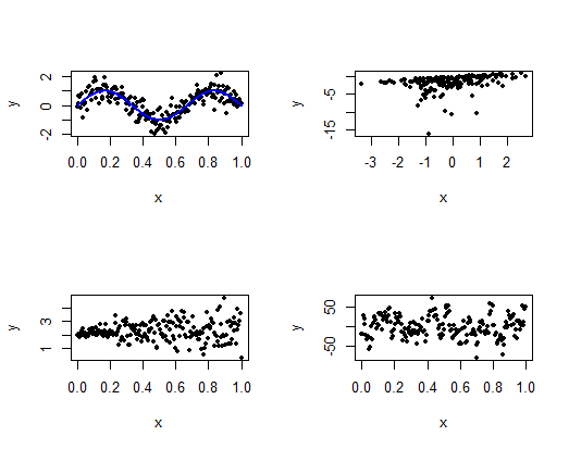
Which assumption is not being satisfied in each of this plots?

2.4 Parameter estimation

2.4.1 Least Squares

Lets go back to the poverty example where \(Y_i\) is the birth rate per 1000 females 15 to 17 years old of \(i^{th}\) State, and \(X_i\) is the poverty index of that State. Consider fitting the best line: \[Bith\;rate_i= \beta_0 +povery \; index_i \,\beta_1+\varepsilon_i\] We could choose among many different lines, 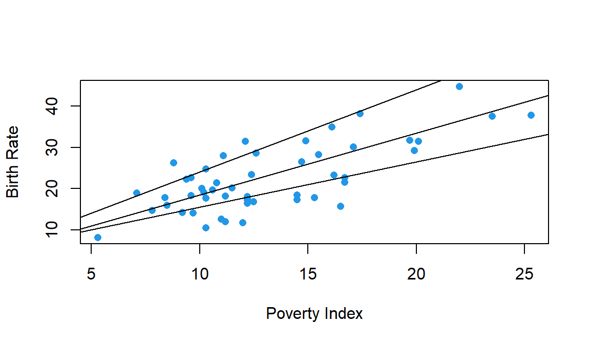The best line will be one that is closest to the points on the scatterplot. In other words, the best line is one that minimizes the total distance between itself and all the observed data points.

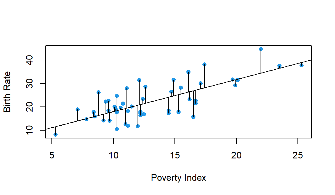
But, why minimise the residual sum of the squares (RSS)? \[RSS(\beta_0,\beta_1)=\sum_{i=1}^n (Y_i-(\beta_0+\beta_1 X_i))^2\] There are other possible objective criteria that could be used. For example, why not just minimise the sum of the absolute deviations of the actual points from the fitted line?
\[\sum_{i=1}^n |Y_i-(\beta_0+\beta_1 X_i)|\] The least squares criteria:

Penalizes more the points that are further from the regression line
It is computationally and mathematically more atractive

In the simple linear regression case, it is well known that the least squares fit yields the following estimates:

\[\hat \beta_1= \frac{S_{xy}}{S_x^2}\quad \hat \beta_0=\overline{Y}- \hat \beta_1 \overline{X}\] where:

\(\overline{Y}\) and \(\overline{X}\) are the sample mean of \(Y\) and \(X\)
\(S_x^2\) is the sample variance of \(X\)
\(S_{xy}\) is the sample covariance between \(X\) and \(Y\)

Exercise 3

Check that for the dataset index.txt, the least squares estimates of the parameters are: \(\hat \beta_0=4.267\) and \(\hat \beta_1=1.373\)

Least Squares in Multiple Regression

When we have more than one covariate, we try to minimize the distance between each point and the hyperplane generated by the covariates

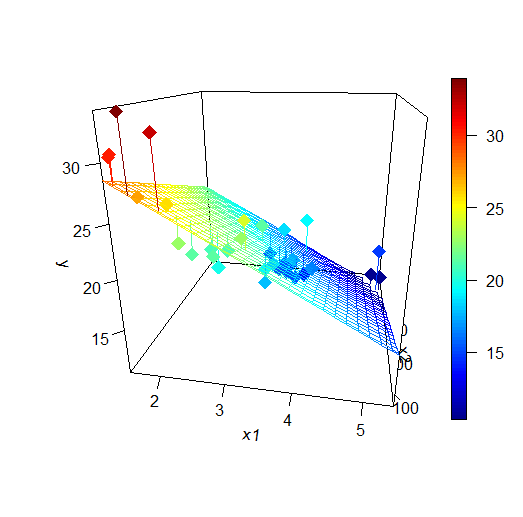
In this case the objective function is: \[RSS(\beta_0,\beta_1, \ldots , \beta_k)=\sum_{i=1}^n (Y_i-(\beta_0+\beta_1 X_{ik}+\ldots + \beta_k x_{ik}))^2\]

Or, in matrix form:

\[\begin{align} RSS(\boldsymbol{\beta})=\left ( \mathbf{Y} -\mathbf{X}\boldsymbol{\beta}\right )^\prime \left ( \mathbf{Y} -\mathbf{X}\boldsymbol{\beta}\right ),\tag{2.2} \end{align}\]

for \(\mathbf{Y}\), \(\mathbf{X}\) and \(\boldsymbol{\beta}\) given in (2.1). In order to calculate the value of the vector of parameters \(\boldsymbol{\beta}\) that minimizes the expression above, we calculate the derivative. using the properties in section 6 given in the Review of Matrix Algebra

\[\frac{\partial RSS}{\partial \boldsymbol{\beta}}=-2\mathbf{X}^\prime \mathbf{Y} +2\mathbf{X}^\prime\mathbf{X} \boldsymbol{\beta}\]

Setting this expression equal to zero, and solving for \(\boldsymbol{\beta}\), we obtain: \[\begin{align} \boldsymbol{\hat \beta}=\left (\mathbf{X}^\prime \mathbf{X}\right )^{-1} \mathbf{X}^\prime \mathbf{Y},\tag{2.3} \end{align}\]

Once the parameters are estimated, we can give expression for the fitted regression line and the estimated (predicted) errors called residuals \[\begin{align} \mathbf{\hat Y}=&\mathbf{X}\left (\mathbf{X}^\prime \mathbf{X}\right )^{-1} \mathbf{X}^\prime \mathbf{Y}=\mathbf{H}\mathbf{Y},\tag{2.4}\\ \boldsymbol{\hat \varepsilon}=&\mathbf{Y}-\mathbf{\hat Y}=\left ( \mathbf{I}-\mathbf{H}\right )\mathbf{Y},\tag{2.5}\\ \end{align}\] \(\mathbf{H}\) is called the Hat Matrix and what it does is to project \(\mathbf{Y}\) into the regression hyperplane.

2.5 Properties of Least Squares

There are several properties of the fitted regression line that will be helpful to understand the relationship between \(\mathbf{X}\), \(\mathbf{Y}\), \(\boldsymbol{\beta}\), and \(\boldsymbol{\varepsilon}\).

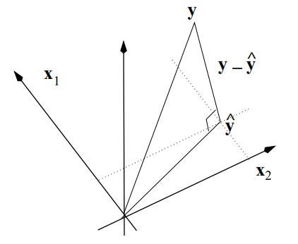
The sum of the residuals is zero: \[\sum_{i=1}^n \hat \varepsilon_i=\mathbf{1}^\prime\left ( \mathbf{I}-\mathbf{H}\right )\mathbf{Y}=0\] -The sum of the observed data is equal to the sum of the fitted values: \[\sum_{i=1}^nY_i=\sum_{i=1}^n\hat Y_i\Rightarrow \mathbf{1}^\prime\mathbf{Y}=\mathbf{1}^\prime\mathbf{\hat Y}\]
The residuals are orthogonal to the preditors \[\sum_{i=1}^n x_i\hat \varepsilon_i=\mathbf{X}^\prime \boldsymbol{\hat \varepsilon}=0\]
The residuals are orthogonal to the fitted values: \[\sum_{i=1}^n \hat y_i\hat \varepsilon_i=\mathbf{\hat Y}^\prime \boldsymbol{\hat \varepsilon}=0\]

2.5.1 Gauss-Markov theorem

Given a multiple regression model in which the hypothesis mentioned earlier are satisfied, then, the least squares estimator \(\boldsymbol{\hat \beta}\) is the best (smallest variance) linear unbiased estimator.

We need to proof that \[Var(\boldsymbol{\tilde \beta}) -Var(\boldsymbol{\hat \beta}) \quad \text{ is positive semidefinite.}\] For that we need to remeber:

\[Var(\boldsymbol{\tilde \beta} -\boldsymbol{\hat \beta})=Var(\boldsymbol{\tilde \beta})+Var(\boldsymbol{\hat \beta}) -2Cov( \boldsymbol{\tilde \beta},\boldsymbol{\hat \beta} ).\]

If \(\boldsymbol{\tilde \beta}\) is another linear estimator of \(\boldsymbol{ \beta}\)\(\Rightarrow\) \(\boldsymbol{\tilde \beta}=\mathbf{C}\mathbf{y}\). If \(\boldsymbol{\tilde \beta}\) is unbiased, then: \[E[\boldsymbol{\tilde \beta}]=\mathbf{C} E(\mathbf{y})=\mathbf{CX}\boldsymbol{\beta} \Rightarrow \mathbf{CX}=\mathbf{I}.\]

We use this result to calculate \(Cov( \boldsymbol{\tilde \beta},\boldsymbol{\hat \beta} )\):

\[Cov( \boldsymbol{\tilde \beta}, \boldsymbol{\hat \beta} )=E[(\boldsymbol{\tilde \beta}-\boldsymbol{ \beta})(\boldsymbol{\hat \beta}- \boldsymbol{\beta})^\prime].\] But, \[ \begin{eqnarray*} \boldsymbol{\tilde \beta} - \boldsymbol{ \beta}&=&\mathbf{Cy}-\boldsymbol{ \beta}=\mathbf{C} (\mathbf{X}\boldsymbol{\beta}+\varepsilon)-\boldsymbol{ \beta}=\mathbf{C} \varepsilon\\ \boldsymbol{\hat \beta} - \boldsymbol{ \beta}&=&(\mathbf{X}^\prime \mathbf{X})^{-1}\mathbf{X}^\prime\mathbf{y}-\boldsymbol{ \beta}=(\mathbf{X}^\prime \mathbf{X})^{-1} \varepsilon. \end{eqnarray*} \]

Then, \[ Cov( \boldsymbol{\tilde \beta}, \boldsymbol{\hat \beta})=E[\mathbf{C}\varepsilon\varepsilon^\prime\mathbf{X}(\mathbf{X}^\prime \mathbf{X})^{-1}]=\sigma^2\mathbf{C}\mathbf{X}(\mathbf{X}^\prime \mathbf{X})^{-1}=\sigma^2(\mathbf{X}^\prime \mathbf{X})^{-1}=Var(\boldsymbol{\hat \beta})\]

Therefore, \[ \begin{eqnarray*} Var(\boldsymbol{\tilde \beta} -\boldsymbol{\hat \beta})&=&Var(\boldsymbol{\tilde \beta})+Var(\boldsymbol{\hat \beta}) -2Cov( \boldsymbol{\tilde \beta}, \boldsymbol{\hat \beta} )\\ &=&Var(\boldsymbol{\tilde \beta})-Var(\boldsymbol{\hat \beta}), \end{eqnarray*}\] then since \(Var(\boldsymbol{\tilde \beta} -\boldsymbol{\hat \beta})\) is positive semidefinite, so it is \(Var(\boldsymbol{\tilde \beta})-Var(\boldsymbol{\hat \beta})\)

2.5.2 Case study application

Remember that the aim was to predict effectively the Hydrostatic measure of percent fat from different covariates. Let’s start by conducting a quick exploratory analysis to have insights into the data:

# Read data
bodyfat <- read.table(file = "./Datasets/bodyfat.txt", header = TRUE)

# Numerical 
summary(bodyfat)
##       age              ht              wt             abs       
##  Min.   :13.00   Min.   :56.00   Min.   : 93.4   Min.   : 6.00  
##  1st Qu.:15.00   1st Qu.:64.56   1st Qu.:125.1   1st Qu.: 9.00  
##  Median :16.00   Median :67.50   Median :142.2   Median :11.00  
##  Mean   :15.72   Mean   :66.79   Mean   :154.1   Mean   :16.73  
##  3rd Qu.:17.00   3rd Qu.:69.00   3rd Qu.:171.3   3rd Qu.:19.00  
##  Max.   :18.00   Max.   :73.00   Max.   :299.2   Max.   :54.00  
##     triceps          subscap          hwfat       
##  Min.   : 6.000   Min.   : 6.00   Min.   : 3.580  
##  1st Qu.: 7.625   1st Qu.: 8.00   1st Qu.: 8.727  
##  Median :10.000   Median : 9.00   Median :11.135  
##  Mean   :12.962   Mean   :12.94   Mean   :14.235  
##  3rd Qu.:14.000   3rd Qu.:12.00   3rd Qu.:15.418  
##  Max.   :42.000   Max.   :43.00   Max.   :41.890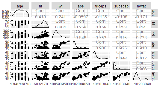

# Graphical - pairwise relations
library(GGally)
ggpairs(bodyfat)

Looking at the plot, it seems that all variables, except perhaps age and height have a strong linear relationship with hydrostatic measure of fat.

There is a strong relationship among several covariates, for example triceps and subscap. This will present a problem when introducing both in the model

It is always a good practice to start by analizing the effect of each covariate separately. The R function to fit linear models is lm()

# hwfat ~ wt
modwt <- lm(hwfat ~ wt, data = bodyfat)

# Summary of the model
summary(modwt)
## 
## Call:
## lm(formula = hwfat ~ wt, data = bodyfat)
## 
## Residuals:
##     Min      1Q  Median      3Q     Max 
## -10.966  -3.701  -1.091   3.019  22.264 
## 
## Coefficients:
##             Estimate Std. Error t value Pr(>|t|)    
## (Intercept) -9.26405    2.59006  -3.577 0.000609 ***
## wt           0.15247    0.01621   9.408 2.22e-14 ***
## ---
## Signif. codes:  0 '***' 0.001 '**' 0.01 '*' 0.05 '.' 0.1 ' ' 1
## 
## Residual standard error: 6.048 on 76 degrees of freedom
## Multiple R-squared:  0.538,  Adjusted R-squared:  0.5319 
## F-statistic:  88.5 on 1 and 76 DF,  p-value: 2.219e-14

The natural step is to include all covariates in order to improve the prediction:

modall <- lm(hwfat ~., data = bodyfat)

# Summary of the model
summary(modall)
## 
## Call:
## lm(formula = hwfat ~ ., data = bodyfat)
## 
## Residuals:
##    Min     1Q Median     3Q    Max 
## -6.162 -1.858 -0.464  2.502  8.177 
## 
## Coefficients:
##             Estimate Std. Error t value Pr(>|t|)    
## (Intercept) 13.29370    9.63027   1.380   0.1718    
## age         -0.32893    0.32158  -1.023   0.3098    
## ht          -0.06731    0.16051  -0.419   0.6762    
## wt          -0.01365    0.02591  -0.527   0.5999    
## abs          0.37142    0.08837   4.203 7.55e-05 ***
## triceps      0.38743    0.13761   2.815   0.0063 ** 
## subscap      0.11405    0.14193   0.804   0.4243    
## ---
## Signif. codes:  0 '***' 0.001 '**' 0.01 '*' 0.05 '.' 0.1 ' ' 1
## 
## Residual standard error: 3.028 on 71 degrees of freedom
## Multiple R-squared:  0.8918, Adjusted R-squared:  0.8827 
## F-statistic: 97.54 on 6 and 71 DF,  p-value: < 2.2e-16

Look at the value of the estimated parameter for wt and compare it with the one in the previuos model. It is quite different!! Why?

A parameter estimate in a regression model (e.g., \(\beta_j\)) will change if a variable, \(\mathbf{X}_j\), is added to the model and:

This will essentially be always the case in practice unless you are working with experimental data where the variables were manipulated such that they are uncorrelated by design.

Exercise 4

Using modall, obtain the model matrix and residuals as:

X=model.matrix(modall)
resid=residuals(modall)

and check that the properties in section 2.5 are satisfied

2.5.3 Maximum Likelihood

The idea of least squares is that we choose parameter estimates that minimize the average squared difference between observed and predicted values. That is, we maximize the fit of the model to the data by choosing the model that is closest, on average, to the data.

The Least Squares’ method does not make any assumptions about the distribution of the response. Although this might be a good thing, it has the drawback that does not allow us to make any inference on the estimated parameters, and therefore, on the predictions.

In maximum likelihood estimation, we search over all possible sets of parameter values for a specified model to find the set of values for which the observed sample was most likely. That is, we find the set of parameter values that, given a model, were most likely to have given us the data that we have in hand.

In the case of linear regression, we search for the set of \(\boldsymbol{\beta}\)’s, given that, \(\mathbf{Y}\sim N\left ( \mathbf{X}\boldsymbol{\beta}, \sigma^2 \mathbf{I}\right )\) that are most likely to have given us the data that we have in hand.

The log-likelihood function is given by:

\[\begin{align*} ln \mathcal{L} (\boldsymbol{\beta},\sigma^2|\mathbf{X})=&\sum_{i=1}^n ln \left (\frac{1}{\sqrt{2\pi\sigma^2}}\right )-\frac{(Y_i-(\beta_0+\beta_1 X_{ik}+\ldots + \beta_k X_{ik}))^2}{2\sigma^2}\\ \propto & -\frac{n}{2}ln(\sigma^2)-\frac{\left ( \mathbf{Y} -\mathbf{X}\boldsymbol{\beta}\right )^\prime \left ( \mathbf{Y} -\mathbf{X}\boldsymbol{\beta}\right )}{2\sigma^2}. \end{align*}\]

Notice that the only part of the equation above that depends on \(\boldsymbol{\beta}\) is the least squares criteria in (2.2). So, minimizing \(-ln \mathcal{L} (\boldsymbol{\beta},\sigma^2|\mathbf{X})\) is equivalent to minimizing least squares.

Estimation of \(\sigma^2\)

Using maximum likelihood we can also estimate \(\sigma^2\)

Unfortunately, this estimator is biased, i.e. \(E[\hat \sigma^2]\neq \sigma^2\). The biased is easily fixed and the unbiased estimator is:

\[\begin{align} \hat \sigma^2=\frac{\left ( \mathbf{Y} -\mathbf{X}\boldsymbol{\hat \beta}\right )^\prime \left ( \mathbf{Y} -\mathbf{X}\boldsymbol{\hat \beta}\right ) }{n-(k+1)} \tag{2.6} \end{align}\]

and \(k+1\) is the number of estimated parameters.

2.5.4 Degrees of freedom

Degrees of freedom refers to the number of independent pieces of information in a sample of data. Since we have estimated \(k+1\) parameters, we have \(n-(k+1)\) information units to estimate \(\sigma^2\). Also, we can see the expression of \(\hat \sigma^2\) given in (2.6) as a sample variance of the residuals (but not divided but the number of observations, but by the number of free observations)

A more general definition of degrees of freedom is given as: \[d.f.=Trace(\mathbf{I}-\mathbf{H})=n-Trace(\mathbf{H})=n-(k+1)\]

2.5.5 Interpretation of the coefficients

Consider the predicted mean for a given set of values of the regressors:

\[E[\mathbf{Y}| \mathbf{X}_1=x_1,\ldots,\mathbf{X}_k=x_k]=\beta_0+\sum_{i=1}^kx_k\beta_k\]

Consider incrementing \(X_1\) by 1:

\[E[\mathbf{Y}| \mathbf{X}_1=x_1+1,\ldots,\mathbf{X}_k=x_k]=\beta_0+\beta_1+\sum_{i=1}^kx_k\beta_k\] Substracting this two equations: \[E[\mathbf{Y}| \mathbf{X}_1=x_1,\ldots,\mathbf{X}_k=x_k]-E[\mathbf{Y}| \mathbf{X}_1=x_1+1,\ldots,\mathbf{X}_k=x_k]=\beta_1\] Then, the interpretation of a multivariate regression coefficient is the expected change in the response per unit change in the regressor, holding all of the other regressors fixed. The latter part of the phrase is important, by holding the other regressors constant, we are investigating an adjusted effect

Let’s illustrate it using the case study. Recall


# Model coefficients
modall
## 
## Call:
## lm(formula = hwfat ~ ., data = bodyfat)
## 
## Coefficients:
## (Intercept)          age           ht           wt          abs      triceps  
##    13.29370     -0.32893     -0.06731     -0.01365      0.37142      0.38743  
##     subscap  
##     0.11405

Now we increase the variable age by 1 year and obtain the predicted values (mantaining the values of the rest of the covariates)

age2=bodyfat$age+1
#create the data.frame for prediction
new=data.frame(age=age2,ht=bodyfat$ht,wt=bodyfat$wt, abs=bodyfat$abs,
               triceps=bodyfat$triceps, subscap=bodyfat$subscap)
#get new fitted values
new.fit=predict(modall,newdata=new)

summary(new.fit-modall$fitted)
##    Min. 1st Qu.  Median    Mean 3rd Qu.    Max. 
## -0.3289 -0.3289 -0.3289 -0.3289 -0.3289 -0.3289

2.6 Inference for model parameters

Recall that the distributional assumptions of the model \(\mathbf{Y}=\mathbf{X}\boldsymbol{\beta} +\boldsymbol{\varepsilon}\) were:

\[\boldsymbol{\varepsilon}\sim N(\mathbf{0},\sigma^2\mathbf{I})\Rightarrow \mathbf{Y}\sim N(\mathbf{X}\boldsymbol{\beta},\sigma^2\mathbf{I} )\]

2.6.1 Sampling distribution of estimated coefficients

Since \(\boldsymbol{\hat \beta}=\left (\mathbf{X}^\prime \mathbf{X}\right )^{-1} \mathbf{X}^\prime \mathbf{Y}\) is a linear combination of the response vector \(\mathbf{Y}\), and \(\mathbf{Y}\) follow a Normal distribution, \(\boldsymbol{\hat \beta}\) is also normally distributed. Therefore, its distribution will be completely specified if we know the mean and variance: \[\begin{align*} E[\boldsymbol{\hat \beta}]=&\left (\mathbf{X}^\prime \mathbf{X}\right )^{-1} \mathbf{X}^\prime E[\mathbf{Y}]=\boldsymbol{\beta}\\ Var[\boldsymbol{\hat \beta}]=&\left (\mathbf{X}^\prime \mathbf{X}\right )^{-1} \mathbf{X}^\prime Var[\mathbf{Y}]\mathbf{X}\left (\mathbf{X}^\prime \mathbf{X}\right )^{-1}=\sigma^2\left (\mathbf{X}^\prime \mathbf{X}\right )^{-1}. \end{align*}\] Therefore: \[\begin{align} \boldsymbol{\hat \beta}\sim N\left (\boldsymbol{\beta}, \sigma^2 \left (\mathbf{X}^\prime \mathbf{X}\right )^{-1} \right ).\tag{2.7} \end{align}\] To gain more insight on the variance of \(\boldsymbol{\beta}\), we use the simple regression case: \(\mathbf{Y}=\beta_0+\beta_1\mathbf{X}_1+\boldsymbol{\varepsilon}\). In this case, the regression matrix \(\mathbf{X}\) has two columns: a colum of 1’s and the column of \(\mathbf{X_1}\). In this case:

\[\left (\mathbf{X}^\prime \mathbf{X}\right )^{-1}=\frac{1}{n \sum_{i=1}^n (x_{1i}-\overline{x}_1)^2}\left [ \begin{array}[h]{cc} \sum_{i=1}^n x_{1i}^2 & -\sum_{i=1}^n x_{1i}\\ -\sum_{i=1}^n x_{1i} &n \end{array} \right ].\]

We can see that the factors involved in the variance of \(\boldsymbol{\hat \beta}\) are:

\(\sigma^2\): The variance of the error
\(n\): the sample size
\((x_{1i}-\overline{x}_1)\): the predictor spread out

So, the smaller the variance of the error, the larger the sample size and the variability of the predictor, the more precise the estimates are.

2.6.2 Confidence intervals/regions for coefficients

A way to express the uncertainty in our estimates is through Confidence Intervals (in the case on a single parameter), i.e., under repeated independent trials, a confidence interval will produce intervals containing the target parameter with probability equal to the level of confidence. From equation (2.7), we know that the distribution for each \(\hat \beta_j\), \(j=0,\ldots, k\) is: \[\hat \beta_j\sim N(\beta_j, \sigma^2 v_{jj}).\] where \(v_{ii}\) is the \(i-th\) element of the diagonal of \(\left (\mathbf{X}^\prime \mathbf{X}\right )^{-1}\). Equivalently:

\[\frac{\hat \beta_j-\beta_j}{\sigma \sqrt{v_{jj}}}\sim N(0, 1).\] However, \(\sigma^2\) will be, in general, unknown, and so we will use an estimate of the variance of \(\hat \beta_j\), \(\widehat{Var(\hat \beta_j)}=\hat \sigma^2\sqrt{v_{jj}}\), and so (check section 6 given in the Review of Matrix Algebra): \[\begin{align} \frac{\hat \beta_j-\beta_j}{\hat \sigma \sqrt{v_{jj}}}\sim t_{n-k-1}. \tag{2.8} \end{align}\] Then, the \((1-\alpha)\%\) confidence interval for \(\hat \beta_j\) is given by:

\[CI_{(1-\alpha)}(\beta_j)=\left [ \hat \beta_j-t_{1-\alpha/2;n-k-1}\hat \sigma \sqrt{v_{jj}}, \hat \beta_j+t_{1-\alpha/2;n-k-1}\hat \sigma \sqrt{v_{jj}} \right ]\]

This is what you obtain we use you use the function confint in an lm object:

confint(modall,level=0.95)
##                   2.5 %      97.5 %
## (Intercept) -5.90850850 32.49590569
## age         -0.97014192  0.31227386
## ht          -0.38735194  0.25273384
## wt          -0.06531058  0.03800691
## abs          0.19522306  0.54761646
## triceps      0.11303958  0.66181336
## subscap     -0.16894384  0.39704811

Looking at the results, we can see that only in two cases (abs and triceps) 0 is not in the confidence interval.

2.6.3 Hypothesis test

The distribution in (2.8), allow us to conduct hypothesis test on the coefficients \(\beta_j\). In the case of linear regression, we normally are interested in testing if the coefficient is equal to 0 or not (significance test), \[H_0: \; \beta_j=0 \quad H_1:\; \beta_j\neq 0\]

In fact, what we are testing is whether the relationship between \(\mathbf{X}_i\) and \(\mathbf{Y}\) is linear or not. The test statistic used is: \[ \frac{|\hat \beta_j-0|}{\widehat{Var[\hat \beta_j]}},\] which is distributed as \(t_{n-k-1}\) under the null hypothesis.

The p-value is a measure of the strength of evidence against the null hypothesis

If p-value is lower than \(\alpha\) \(\rightarrow\) Reject \(H_0\)
If p-value is greater than \(\alpha\) \(\rightarrow\) Do not reject \(H_0\)

2.6.4 Case study application

When you run summary on the output of modall, part of what it delivers is a table containing:

Estimate: Estimated coefficients, \(\hat \beta_j\)
Std. Error: Estimated standar error of the coefficient, \(\hat \sigma\sqrt{v_{ii}}\)
t value: Test statistic, \(\frac{\hat \beta_j}{\sigma\sqrt{v_{jj}}}\)
Pr(>|t|): p-value

summary(modall)
## 
## Call:
## lm(formula = hwfat ~ ., data = bodyfat)
## 
## Residuals:
##    Min     1Q Median     3Q    Max 
## -6.162 -1.858 -0.464  2.502  8.177 
## 
## Coefficients:
##             Estimate Std. Error t value Pr(>|t|)    
## (Intercept) 13.29370    9.63027   1.380   0.1718    
## age         -0.32893    0.32158  -1.023   0.3098    
## ht          -0.06731    0.16051  -0.419   0.6762    
## wt          -0.01365    0.02591  -0.527   0.5999    
## abs          0.37142    0.08837   4.203 7.55e-05 ***
## triceps      0.38743    0.13761   2.815   0.0063 ** 
## subscap      0.11405    0.14193   0.804   0.4243    
## ---
## Signif. codes:  0 '***' 0.001 '**' 0.01 '*' 0.05 '.' 0.1 ' ' 1
## 
## Residual standard error: 3.028 on 71 degrees of freedom
## Multiple R-squared:  0.8918, Adjusted R-squared:  0.8827 
## F-statistic: 97.54 on 6 and 71 DF,  p-value: < 2.2e-16

It is important to be very clear about the hypothesis being tested here. There is in fact a different null hypothesis for each row of the table. The null hypothesis for \(\beta_j\) is:

\[H_0: \; \mathbf{Y}=\beta_0 +\mathbf{X}_{1}\beta_1+\ldots +\mathbf{X}_{i-1}\beta_{i-1}+\mathbf{X}_{i+1}\beta_{i+1}+\ldots+\mathbf{X}_{k}\beta_k+\boldsymbol{\varepsilon}\]

This matters because whether the null hypothesis is true or not depends on what other variables are included in the model.

To illustrate that, recall the model modwt (that included only weight as a covariate)

summary(modwt)
## 
## Call:
## lm(formula = hwfat ~ wt, data = bodyfat)
## 
## Residuals:
##     Min      1Q  Median      3Q     Max 
## -10.966  -3.701  -1.091   3.019  22.264 
## 
## Coefficients:
##             Estimate Std. Error t value Pr(>|t|)    
## (Intercept) -9.26405    2.59006  -3.577 0.000609 ***
## wt           0.15247    0.01621   9.408 2.22e-14 ***
## ---
## Signif. codes:  0 '***' 0.001 '**' 0.01 '*' 0.05 '.' 0.1 ' ' 1
## 
## Residual standard error: 6.048 on 76 degrees of freedom
## Multiple R-squared:  0.538,  Adjusted R-squared:  0.5319 
## F-statistic:  88.5 on 1 and 76 DF,  p-value: 2.219e-14

In this case we do reject the null hypothesis (the parameter for weight is 0), while in modall we do not reject that hypothesis. Why is that?

What happened with the variable wt is that it added little information to the response, once the other variables are included in the model. This is due to the fact that there is a very high correlation between wt and the other predictors, and so, the information is already provided by the other predictor, this is called Multicollinearity.

A good practice is to calculate the pairwise correlation between the covariates

round(cor(model.matrix(modall)[,-1]),2)
##           age   ht   wt   abs triceps subscap
## age      1.00 0.42 0.24 -0.06   -0.13   -0.11
## ht       0.42 1.00 0.60  0.26    0.16    0.25
## wt       0.24 0.60 1.00  0.85    0.75    0.81
## abs     -0.06 0.26 0.85  1.00    0.91    0.93
## triceps -0.13 0.16 0.75  0.91    1.00    0.95
## subscap -0.11 0.25 0.81  0.93    0.95    1.00

The hight correlation between wt, abs,triceps and subscap is an indication that we are including redundant information.

The reason why the coefficients become non-significant is because the variance of the estimates is inflated and the estimates might even have the wrong sign (as it happens with wt).

Ways to deal with multicollinearity:

Ignore it. If prediction of y values is the object of your study, then collinearity is not a problem
Use an estimator of the regression coefficients other than the least squares estimators. An alternative is to use ridge regression estimators (we will se this later in the course)
Get rid of the redundant variables by using a variable selection technique

2.6.5 ANOVA

The linear regression model can also be considered in what is called Analisis of Variance framework. This new paradigm will be useful when working with multiple regression model. A way to think about regression is in the decomposition of variability of our response.

The total variability in our response is the variability around an intercept. This is also the variance estimate from a model with only an intercept:

\[ Total \; variability = \sum_{i=1}^n \left (Y_i-\overline{\mathbf{Y}}\right )^2\]

The regression variability is the variability that is explained by adding the predictors. Mathematically, this is:

\[ Regression \; variability = \sum_{i=1}^n \left ( \hat Y_i-\overline{\mathbf{Y}}\right )^2\] The residual variability is what is leftover around the regression line

\[ Residual \; variability = \sum_{i=1}^n \left ( Y_i-\hat Y_i\right )^2\] It is an important fact that the error and regression variability add up to the total variability:

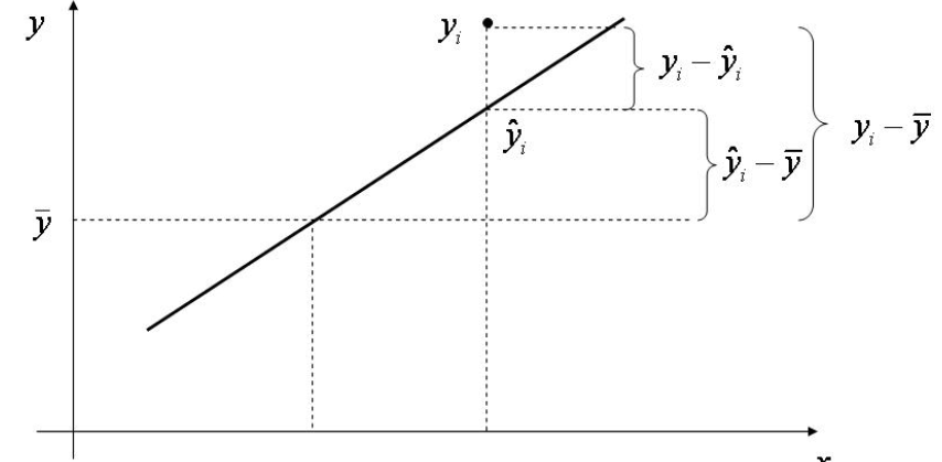\[\begin{align} \underbrace{\sum_{i=1}^n \left (Y_i-\overline{\mathbf{Y}}\right )^2}_{SST}= \underbrace{\sum_{i=1}^n \left ( \hat Y_i-\overline{\mathbf{Y}}\right )^2}_{SSR} +\underbrace{\sum_{i=1}^n \left ( Y_i-\hat Y_i\right )^2}_{SSE} \tag{2.9} \end{align}\] Thus, we can think of regression as explaining away variability.

The fact that all of the quantities are positive and that they add up allows us to define the proportion of the total variability explained by the model.

Exercise 5

Proof the equality in equation (2.9).

This decomposition will help us to test hypothesis such us:

\[H_0: \beta_1=0, \ldots, \beta_k=0 \quad H_1: At \; least\; one \; \beta_j\neq 0\]

This is called F-test and, if \(H_0\) is rejected, we will conclude that at least one \(\beta_j\) is significantly different from zero. An intuitive way to carry out the test would be to compare SST and SSR. However we can’t compare them directly, but it happens that, under \(H_0\):

\[F=\frac{SSR/k}{SSE/(n-k-1)}\sim F_{k,n-k-1}\] This can be summarized in the following table calle the ANOVA table:

	Degrees of freedom	Sum Squares	Mean Squares	\(F\)-value	\(p\)-value
Regression	\(k\)	SSR	\(\frac{\text{SSR}}{k}\)	\(\frac{\text{SSR}/k}{\text{SSE}/(n-k-1)}\)	\(p\)
Residuals	\(n-k-1\)	SSE	\(\frac{\text{SSE}}{n-k-1}\)

This test appears in the summary of the lm objects

summary(modall)
## 
## Call:
## lm(formula = hwfat ~ ., data = bodyfat)
## 
## Residuals:
##    Min     1Q Median     3Q    Max 
## -6.162 -1.858 -0.464  2.502  8.177 
## 
## Coefficients:
##             Estimate Std. Error t value Pr(>|t|)    
## (Intercept) 13.29370    9.63027   1.380   0.1718    
## age         -0.32893    0.32158  -1.023   0.3098    
## ht          -0.06731    0.16051  -0.419   0.6762    
## wt          -0.01365    0.02591  -0.527   0.5999    
## abs          0.37142    0.08837   4.203 7.55e-05 ***
## triceps      0.38743    0.13761   2.815   0.0063 ** 
## subscap      0.11405    0.14193   0.804   0.4243    
## ---
## Signif. codes:  0 '***' 0.001 '**' 0.01 '*' 0.05 '.' 0.1 ' ' 1
## 
## Residual standard error: 3.028 on 71 degrees of freedom
## Multiple R-squared:  0.8918, Adjusted R-squared:  0.8827 
## F-statistic: 97.54 on 6 and 71 DF,  p-value: < 2.2e-16

Of course, this decomposition of the variance can be used to test whether one, or a group of coefficients is zero. This is based on what is known as extra sum of squares, and it measures the marginal increase in regression sum of squares when one or more variables are added to the regression model. For example, in the case of only two predictors \(\mathbf{X}_1\) and \(\mathbf{X}_2\). The marginal increse when adding \(\mathbf{X}_2\) to a model that already has \(\mathbf{X}_1\) is given by:

\[ SSR(\mathbf{X}_2|\mathbf{X}_1)=SRR(\mathbf{X}_2,\mathbf{X}_1)-SSR(\mathbf{X}_1)\] When the model has \(k\) variables, there are \(k!\) possible decompositions of the variability. In the case of k=3, there are 6 decompositions: \[ \begin{aligned} SSR(\mathbf{X}_1,\mathbf{X}_2,\mathbf{X}_1) &= SSR(\mathbf{X}_1)+SSR(\mathbf{X}_2|\mathbf{X}_1)+SSR(\mathbf{X}_3|\mathbf{X}_1,\mathbf{X}_2)\\ SSR(\mathbf{X}_1,\mathbf{X}_3,\mathbf{X}_2) &= SSR(\mathbf{X}_1)+SSR(\mathbf{X}_3|\mathbf{X}_1)+SSR(\mathbf{X}_2|\mathbf{X}_1,\mathbf{X}_3)\\ SSR(\mathbf{X}_2,\mathbf{X}_1,\mathbf{X}_3) &= SSR(\mathbf{X}_2)+SSR(\mathbf{X}_1|\mathbf{X}_2)+SSR(\mathbf{X}_2|\mathbf{X}_1,\mathbf{X}_2)\\ & \vdots\\ \end{aligned} \]

2.6.6 Case study application

The function in R to calculate the analysis of variance table is anova() and the input is one or more lm objects. If the input is one model:

#ANOVA Table for model `modall`
anova(modall)
## Analysis of Variance Table
## 
## Response: hwfat
##           Df Sum Sq Mean Sq  F value    Pr(>F)    
## age        1  175.0   175.0  19.0863 4.180e-05 ***
## ht         1  325.0   325.0  35.4466 9.096e-08 ***
## wt         1 3953.8  3953.8 431.1764 < 2.2e-16 ***
## abs        1  719.5   719.5  78.4697 4.290e-13 ***
## triceps    1  187.5   187.5  20.4433 2.400e-05 ***
## subscap    1    5.9     5.9   0.6458    0.4243    
## Residuals 71  651.0     9.2                       
## ---
## Signif. codes:  0 '***' 0.001 '**' 0.01 '*' 0.05 '.' 0.1 ' ' 1

In the first line, the models being tested are: \[H_0: \mathbf{Y}=\beta_0+\boldsymbol{\varepsilon}\quad H_1: \mathbf{Y}=\beta_0+\beta_1age+\boldsymbol{\varepsilon}\] In the second line: \[H_0: \mathbf{Y}=\beta_0+\beta_1age+\boldsymbol{\varepsilon}\quad H_1: \mathbf{Y}=\beta_0+\beta_1 age+\beta_2ht+\boldsymbol{\varepsilon},\] and so on. Therefore, the sum of squares reported are the conditional sum of squares (conditional on the previous predictors being in the model). For example \(325=SSR(ht|age)=SSR(age,ht)-SSR(age)\).

Do you find something surprising when you compare the output of summary and anova for modall?

IMPORTANT: The order of the variables specified in the model impact the ANOVA table in R. You need to be carefull when predictors are correlated!!

Let’s change the order of the variables in the model:

#Model with all variables in different order
modall2=lm(hwfat~triceps+abs+subscap+wt+ht+age, data=bodyfat)
#results from the both methods
summary(modall2)
## 
## Call:
## lm(formula = hwfat ~ triceps + abs + subscap + wt + ht + age, 
##     data = bodyfat)
## 
## Residuals:
##    Min     1Q Median     3Q    Max 
## -6.162 -1.858 -0.464  2.502  8.177 
## 
## Coefficients:
##             Estimate Std. Error t value Pr(>|t|)    
## (Intercept) 13.29370    9.63027   1.380   0.1718    
## triceps      0.38743    0.13761   2.815   0.0063 ** 
## abs          0.37142    0.08837   4.203 7.55e-05 ***
## subscap      0.11405    0.14193   0.804   0.4243    
## wt          -0.01365    0.02591  -0.527   0.5999    
## ht          -0.06731    0.16051  -0.419   0.6762    
## age         -0.32893    0.32158  -1.023   0.3098    
## ---
## Signif. codes:  0 '***' 0.001 '**' 0.01 '*' 0.05 '.' 0.1 ' ' 1
## 
## Residual standard error: 3.028 on 71 degrees of freedom
## Multiple R-squared:  0.8918, Adjusted R-squared:  0.8827 
## F-statistic: 97.54 on 6 and 71 DF,  p-value: < 2.2e-16
anova(modall2)
## Analysis of Variance Table
## 
## Response: hwfat
##           Df Sum Sq Mean Sq  F value    Pr(>F)    
## triceps    1 5056.3  5056.3 551.4078 < 2.2e-16 ***
## abs        1  258.8   258.8  28.2184 1.187e-06 ***
## subscap    1    2.2     2.2   0.2447   0.62237    
## wt         1   38.0    38.0   4.1444   0.04551 *  
## ht         1    1.9     1.9   0.2065   0.65091    
## age        1    9.6     9.6   1.0463   0.30984    
## Residuals 71  651.0     9.2                       
## ---
## Signif. codes:  0 '***' 0.001 '**' 0.01 '*' 0.05 '.' 0.1 ' ' 1

The output of summary is the same as before, since in each line we are testing the model without the variable in question against the model in all variables, while in the anova case is different because the sum of squares are calculated conditioning on different variables. So, how can we use the anova function to test whether a predictor is relevant, provided that the rest remain in the model? To do so we include in the fuction anova the model under the null and the alternative hypothesis.

#Anova table to test whether  `age` should be in the model
#The input is the model without and with `age`
anova(update(modall,.~.-age), modall2)
## Analysis of Variance Table
## 
## Model 1: hwfat ~ ht + wt + abs + triceps + subscap
## Model 2: hwfat ~ triceps + abs + subscap + wt + ht + age
##   Res.Df    RSS Df Sum of Sq      F Pr(>F)
## 1     72 660.64                           
## 2     71 651.05  1     9.594 1.0463 0.3098

In this case the output of the table is a bit different

The second column gives \(SSE\) for each model (here, \(SSE\) is also called Residual sum of squares (\(RSS\)))
The thrid column gives the conditional \(SSR\) for age, given that all another variables are in the model

\[ \small \underbrace{SSR(age|ht,wt,abs,triceps,subscap)}_{9.594}=\underbrace{SSE(ht,wt,abs,triceps,subscap)}_{660.64}\\ -\underbrace{SSE(age,ht,wt,abs,triceps,subscap)}_{651.05}\]

Exercise 6

Test if each coefficient is significant (conditional on all other variables being in the model) using the anova function, and compare the results with the output summary

Use also the anova function to test whether age and ht can be dropped simultaneously from the model

Coefficient of Determinarion \(R^2\)

The fact that all of the quantities in the sum of squares decomposition, \(SST=SSR+SSE\), are positive and that they add up, allows us to define the proportion of the total variability explained or not by the model. Therefore, the ratio \(\frac{SSE}{SST}\) represents the proportion of variability that cannot be explained by the model, and the coefficient of determination is defined as the proportion of variability explained by the model

\[R^2=1-\frac{SSE}{SST}=\frac{SSR}{SST}\]

\(0\leq R^2 \leq 1\)
Increases as more variables are included in the model

It is possible to get a negative \(R^2\) for equations that do not contain a constant term. Because \(R^2\) is defined as the proportion of variance explained by the fit, if the fit is actually worse than just fitting a horizontal line then R-square is negative. Such situations indicate that a constant term should be added to the model.

This last point is a disadvantaje if we want to use \(R^2\) as a measure of the goodness of fit of a model (or to find the simplest model with the largest value of \(R^2\)), since, even if the variable are non-significant, their inclusion in the model will increase \(R^2\). To avoid that effect we need a measure that takes into account the number of variables included in the model. Such a measure is the Adjusted coefficient of determination which is computed by dividing each sum of squares by its associated degrees of freedom:

\[R^2_a=1-\frac{\frac{SSE}{n-k-1}}{\frac{SST}{n-1}}=1-\frac{\hat \sigma^2}{SST}\times (n-1)\]

# R^2 for model with all variables except subscap
summary(update(modall, .~.-subscap))$r.squared
## [1] 0.8908285

# R^2 for model with all variables 
summary(modall)$r.squared
## [1] 0.8918125

# Adjusted R^2 for model with all variables except subscap
summary(update(modall, .~.-subscap))$adj.r.squared
## [1] 0.8832472

# Adjusted R^2 for model with all variables 
summary(modall)$adj.r.squared
## [1] 0.8826699

In this case including the predictor subscap increases \(R^2\) from \(0.8908285\) to \(0.8918125\). However, the reduction in \(SSE\) does not compensate the increse in one degree of freedon, and so the \(R^2_a\) descreases from \(0.8832472\) to \(0.8826699\).

\(R^2_a\) is normally used as a goodness of measure. But:

It can be arbitrarily low when the model is completely correct (making \(\sigma^2\) large, even when every assumption of the regression model is correct).
It can be arbitrarily close to 1 when the model is totally wrong.

\(R^2_a\) is a handy, seemingly intuitive measure of how well your linear model fits the data. However, it does not tell us the entire story. You should evaluate \(R^2_a\) values in conjunction with model diagnostics

Let’s see a couples of examples in which \(R^2_a\) does not reflects the model behind the data:

#Generate data with large variabilty
x <- 1:20                        
set.seed(2)                      
y <- 2 + 0.5*x + rnorm(20,0,4) 
#Fit the model
mod <- lm(y~x)                   
summary(mod)$adj.r.squared 
## [1] 0.3386976
plot(x,y)
abline(mod)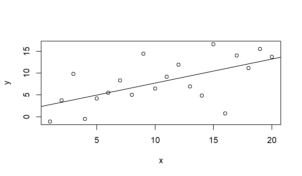

set.seed(1)
 # non-linear data generation
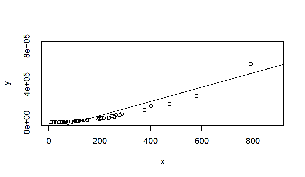
x <- rexp(50,rate=0.005)                     
y <- (x-1)^2 * runif(50, min=0.8, max=1.2)  
mod=lm(y ~ x)
#still a good $r2$
summary(mod)$adj.r.squared
## [1] 0.8453587
plot(x,y)
abline(mod)