Chapter 6 Models for binary data
Before we give a general description of the Generalized Linear Models (glms) we will focus on some of the most relevant cases, as is the case of logistic regression
6.1 Introduction
Recall that in the linear regression model: \[Y_i =\beta_0 +\beta_1 x_{i1} +\beta_2 x_{i2}+\ldots \beta_k x_{ik}+\varepsilon_i,\] the response \(Y_i\) is modelled by a linear function of the predictors plus an error term. We also assumed that, \[\varepsilon_i\sim N(0,\sigma^2)\] Although this is a very useful framework, there are some situations where linear models are not appropriate:
- the range of Y is restricted (e.g. binary, count)
- the variance of Y depends on the mean
Generalized linear models extend the general linear model framework to address both of these issues.
Suppose we have a binary response variable (0 or 1), and we model the response as (we assume a single predictor for simplicity): \[Y_i =\beta_0 +\beta_1 x_{i}+ \varepsilon_i,\] we assume that the response variable is Bernouilli with the following probability function: \[Pr(Y_i=0)=1-p_i \quad Pr(Y_i=1)=p_i.\] Now, since the expected value of a Bernouilli distribution is \(p_i\) and \(E[\varepsilon_i]=0\). Then, \[p_i=E[Y_i|x_i]=\beta_0+\beta_1x_i.\] There are some very basic problems with this regression model. First, if the response is binary, then, the error term can only take on two values: \[\begin{aligned} \varepsilon_i=&1-\beta_0+\beta_1x_i & Y_i=1 \\ \varepsilon_i=&\beta_0+\beta_1x_i & Y_i=0\\ \end{aligned}\] Therefore, the errors in this model cannot be normal. Also, the variance is not constant: \[Var[Y_i]=p_i(1-p_i),\] and \(p_i=E[Y_i]=\beta_0+\beta_1x_i\). Then, the variance is a function of the mean. Finally, there is a constraint on the response function, because \[0\leq E[Y_i]=p_i \leq 1\] This restriction can cause serious problems with the choice of a linear response function. It would be possible to fit a model to the data for which the predicted values of the response lie outside the \([0, 1]\) interval.
It is problematic to apply least-squares linear regression to a dichotomous response variable:
- The errors cannot be normally distributed and cannot have constant variance.
- The linear specification does not confine the probability for the response to the unit interval
6.2 Case study: Health perception survey Comunidad de Madrid

Self-perceived health is a health measure with well-established links with functional status, morbidity, and mortality and is an important measure in determining health-related quality of life, healthcare services utilization, and future health. Therefore it is of interest to see what are the variables that affect self-perceived heath. The data correspond to 7357 individuals that were interviewed between 2001 and 2004 and ask about their sef-perceived heath and personal characteristics and habits
health <- read.table(file = "./Datasets/health.txt", header = TRUE)
knitr::kable(
  head(health, 10),
  booktabs = TRUE,
  longtable = TRUE,
  caption = 'First 10 rows of the `heath` dataset.'
)| sex | g01 | g02 | weight | height | con_tab | year | educa | imc | drink | age |
|---|---|---|---|---|---|---|---|---|---|---|
| 1 | 2 | 1 | 67 | 165 | 1 | 2002 | 4 | 24.61 | 1 | 25 |
| 1 | 2 | 1 | 76 | 166 | 2 | 2004 | 2 | 27.58 | 1 | 43 |
| 1 | 2 | 1 | 77 | 178 | 2 | 2002 | 4 | 24.30 | 1 | 29 |
| 1 | 2 | 1 | 75 | 175 | 1 | 2002 | 3 | 24.49 | 1 | 35 |
| 1 | 1 | 1 | 76 | 177 | 2 | 2003 | 4 | 24.26 | 1 | 38 |
| 1 | 2 | 1 | 84 | 174 | 1 | 2003 | 4 | 27.74 | 1 | 50 |
| 1 | 1 | 1 | 94 | 197 | 1 | 2002 | 3 | 24.22 | 1 | 26 |
| 1 | 1 | 1 | 78 | 178 | 1 | 2003 | 3 | 24.62 | 1 | 29 |
| 1 | 1 | 1 | 65 | 162 | 1 | 2001 | 4 | 24.77 | 1 | 28 |
| 1 | 1 | 1 | 75 | 172 | 1 | 2003 | 3 | 25.35 | 0 | 22 |
The variable are:
age: Age in yearsheight: Height in cmsweight: Weight in kgsyear: Year in which the data was recordeddrink: Categorical variable (to be defined as a factor) with levels0,1and2(no drink, occasional, frequent)sex: Categorical variable (to be defined as a factor) with levels1and2(male, female)con_tab: Categorical variable (to be defined as a factor) with levels1and2(non or occasional smoker, frequent smoker)educa: Categorical variable (to be defined as a factor) with levels1,2,3and4indicating the level of education (low, low-median, median-high, high)imc: Body mass indexg02: The response variable, takes values1and0(good health or no good health)
We will start by focusing on the response variable g02 and three predictots: sex, age and drink.
#Start by defining the categorical variables as factors
health$drink=factor(health$drink)
health$sex=factor(health$sex)
#Summary of the data
library(faraway)
summary(health[,c("g02","sex","age","drink")])
## g02 sex age drink
## Min. :0.0000 1:3666 Min. :18.00 0:2977
## 1st Qu.:1.0000 2:3691 1st Qu.:28.00 1:4054
## Median :1.0000 Median :39.00 2: 326
## Mean :0.8089 Mean :39.24
## 3rd Qu.:1.0000 3rd Qu.:49.00
## Max. :1.0000 Max. :64.00The response can be coded as 0s or 1s or as a factor with two level
#plot response versus age
par(mfrow=c(1,2))
plot(health$age, health$g02, xlab="Age", ylab="Health")
plot(jitter(g02,0.1) ~ jitter(age), health, xlab="Age", ylab="Health",
pch=".")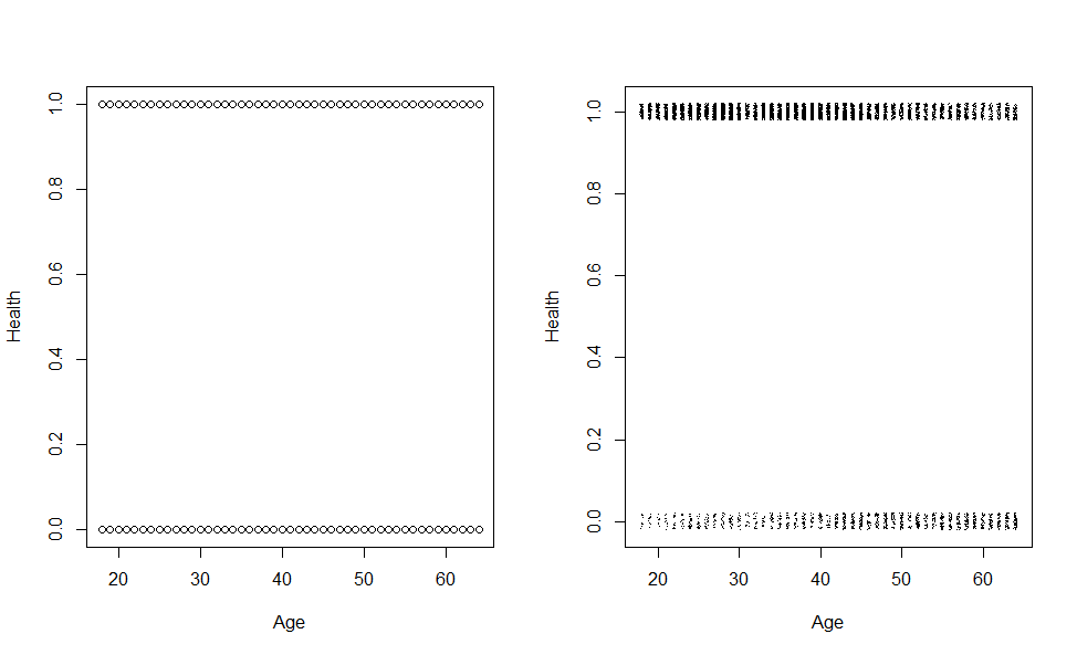 On the left panel is the results of plotting the response versus age. Since there are several people with the same outcome and age it is not possible to see that in the plot. To avoid that to add a
small amount of noise to each point, called jittering, so that we can distinguish them (the result is the plot on the right hand side). Attempting to fit a straight line through this data would be an important mistake.
6.3 Logistic Regression
Suppose we have a response variable \(Y_i\) for \(i = 1, \ldots ,n\) which takes the values zero or one with \((Y_i = 1) = p_i\). This response may be related to a set of \(k\) predictors. We need a model that describes the relationship of the predictors to the probability \(p_i\). Following the linear model approach, we construct a linear predictor: \[\eta_i=\beta_0 +\beta_1 x_{i1} +\beta_2 x_{i2}+\ldots \beta_k x_{ik}\] We have seen previously that the linear relation \(\eta_i = p_i\) is not workable because we require \(0 \leq p_i \leq 1\). Instead we shall use a link function \(g\) such that \(\eta_i = g(p_i)\). We need \(g\) to be monotone and be such that \(0 \leq g^{-1}(\eta) \leq 1\) for any \(\eta\). The most popular choice of link function in this situation is the logit. \[ \eta=log\left ( \frac{p}{1-p}\right ) \Rightarrow p=\frac{e^\eta}{1+e^\eta}\]
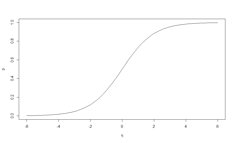
The logistic curve is almost linear in its midrange. This means that for modeling responses that are all of moderate probability, logistic and linear regression will not behave very differently. The curve approaches one at its upper end and zero at its lower end but never reaches these bounds. This means that logistic regression will never predict that anything is inevitable or impossible. It maps \(p\), which is bounded between 0 and 1, to the real number line. The ratio \(p/(1 - p)\) in the transformation is called the odds. Sometimes the logit transformation is called the log-odds.
6.3.1 Other link functions
Besides the logit function, there are other two link functions that are used when modelling binary/binomial data:
- Probit: \(\eta=\Phi^{-1}(p)\) where \(\Phi()\) is the distribution function of a standard Normal random variable
- Complementary log-log: \(\eta=log(-log(1-p))\)
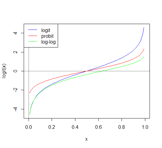 It is usually not
possible to choose the appropriate link function based on the data alone. For regions of moderate \(p\), that is
not close to zero or one, the link functions are quite similar and so a
very large amount of data would be necessary to distinguish between them. Larger
differences are apparent in the tails, but for very small \(p\), one needs a very large amount of data to obtain just a few successes, making it expensive to distinguish between link
functions in this region.
Usually, the choice of link function is made based on assumptions derived from physical knowledge or simple convenience
6.4 Parameter Estimation
We have already shown why it is not appropriate the use of least squares when modelling a binary response, therefore, we will need to use maximum likelihood.
Since each observation \(Y_i\) is assumed to follow a Bernouilli distribution, the probability distribution is given by: \[f(Y_i)=p_i^{Y_i} (1-p_i)^{1-Y_i} \quad i=1, \ldots , n\] The likelihood function is given by: \[\mathcal{L}(y_1,\ldots , y_n)=\prod_{i=1}^n p_i^{Y_i} (1-p_i)^{1-Y_i},\] and the log-likelihood: \[log\,\mathcal{L}(y_1,\ldots , y_n)=\sum_{i=1}^n {Y_i}log (p_i) +(1-Y_i)log (1-p_i)=\sum_{i=1}^n \left [ Y_i log \left ( \frac{p_i}{1-p_i}\right )\right ]+\sum_{i=1}^n log (1-p_i),\] We know that:
- \(\eta_i=log \left ( \frac{p_i}{1-p_i}\right )=\beta_0+\beta_1 x_{i1} +\beta_2 x_{i2}+\ldots \beta_k x_{ik}=\mathbf{X}_i \boldsymbol{\beta}\)
- \(p_i=\frac{e^{\eta_i}}{1+e^{\eta_i}}\Rightarrow 1-p_i=\frac{1}{1+e^{\eta_i}}\Rightarrow log (1-p_i)=-log (1+e^{\eta_{i}})=-log(1+\mathbf{X_i} \boldsymbol{\beta})\)
then, we can express the log-likelihood in terms of the response and the coefficients in the linear predictor: \[log \mathcal{L}(\boldsymbol{\beta};\mathbf{Y})=\sum_{i=1}^n Y_i\mathbf{X}_i\boldsymbol{\beta}-\sum_{i=1}^n log \left [ 1+e^{\mathbf{x}_i^\prime \boldsymbol{\beta}} \right ] \] Unfortunately, the equation \(\frac{\partial log \mathcal{L}(\boldsymbol{\beta};\mathbf{Y})}{\partial \boldsymbol{\beta}}=0\) has no analytic solution, a possible solution is to use an approximation via Newton-Rapson algorithm (as we saw in the previuos chapter).
In R, the function to use logistic regression (and in general any glm) is the glm()function whose main arguments are:
formula: similar to the one used in linear modelsfamily: indicating the probability distribution of the response (defaul option is normal, other options are: biThe model we have fitted is: \[log \left ( \frac{\hat p}{1-\hat p} \right )=1.27-0.24\times sex_{female} + 0.55 \times bebedor_{occasional} + 0.49\times bebedor_{frequent}\]nomial, poisson, gamma, etc.)link: the link function we want to use (in the case of the binomial distribution, the default link is the logit)
# Logistic Regression using sex and drink
lmod <- glm(g02 ~ sex + drink, family = binomial, health)
summary(lmod)
##
## Call:
## glm(formula = g02 ~ sex + drink, family = binomial, data = health)
##
## Coefficients:
##             Estimate Std. Error z value Pr(>|z|)
## (Intercept)  1.26858    0.06027  21.049  < 2e-16 ***
## sex2        -0.23868    0.06230  -3.831 0.000128 ***
## drink1       0.55151    0.06288   8.771  < 2e-16 ***
## drink2       0.49377    0.15984   3.089 0.002007 **
## ---
## Signif. codes:  0 '***' 0.001 '**' 0.01 '*' 0.05 '.' 0.1 ' ' 1
##
## (Dispersion parameter for binomial family taken to be 1)
##
##     Null deviance: 7177.9  on 7356  degrees of freedom
## Residual deviance: 7059.2  on 7353  degrees of freedom
## AIC: 7067.2
##
## Number of Fisher Scoring iterations: 4
6.4.1 Parameter interpretation
An important distinction between linear and logistic regression is that the regression coefficients in logistic regression are not directly meaningful. Before we can interpret the coefficients, we need to recall the meaning of Odds: \[Odds=\frac{p}{1-p} \] Odds are not a probability, but they are very close if the probability is small. If we know the odds we can calculate the probability according to: \(odds/(1 + odds)\).
Suppose we have a logistic regression model with a single predictor, the estimated linear predictor at a particular value of the covariate (\(x_i\)) will be: \[\hat \eta(x_i)=\hat \beta_0+\hat \beta_1x_i=log \left ( \frac{\hat p_i}{1-\hat p_i}\right )=log(odds_{x_i})\]
In linear regression, a value of \(\hat \beta_1=1\) means that if you change \(x_i\) by \(1\), the expected value of the response will go up by \(1\)
In logistic regression, since the linear predictor is the log-odds: a value of \(\hat \beta_1=1\) means that if you change \(x_i\) by 1, the \(log\) of the odds that \(Y\) occurs will go up by 1 (much less interpretable), When interpreting parameters in logistic regression we have to consider:
- The functional relationship between the dependent variable and independent variable/s
- The unit of change of the independent variable/s
The interpretation also will depend on the type of independent variables: dichotomous, polytomous or continuous.
Dichotomous independent variable
Let us first consider the case where the predictor \(X\) is categorical with two levels (0 and 1)
The model is:
\[log \left ( \frac{p}{1-p}\right )=\beta_0+\beta_1X,\]
the difference in the logit for an individual such that \(X = 0\) or \(X=1\) is \(\beta_1\). Also:
\[p=\frac{e^{\beta_0+\beta_1X}}{1+e^{\beta_0+\beta_1X}}\quad 1-p=\frac{1}{1+e^{\beta_0+\beta_1X}}\]
The different values for the probabilities and all possible combinations are:
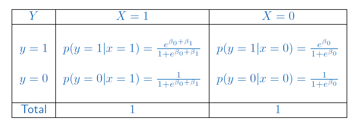
Then, the odds-ratio (OR) is the ratio of the odds of an event occurring in one group to the odds of it occurring in another group: \[OR=\frac{p(y=1|x=1)/1-p(y=1|x=1)}{p(y=1|x=0)/1-p(y=1|x=0)}\] The \(OR\) is one way to quantify how strongly the level of the factor is associated with the presence or absence of property measured in the response in a given population. A value of the \(OR=1\) means that both levels of the categorical variable have similar impact on the response. An \(OR\) less than 1 means that the outcome is less frequent in factor-level of interest than in the factor-level taken as reference (and conversely for \(OR>1\)).
Using the previous table: \[OR =\frac{\left .\left ( \frac{e^{\beta_0+\beta_1}}{1+e^{\beta_0+\beta_1}}\right )\right /\left ( \frac{1}{1+e^{\beta_0+\beta_1}}\right )}{\left .\left ( \frac{e^{\beta_0}}{1+e^{\beta_0}}\right )\right /\left ( \frac{1}{1+e^{\beta_0}}\right )}= \frac{e^{\beta_0+\beta_1}}{e^{\beta_0}}= e^{\beta_1}\] The \(OR\) is not to be confused with relative risk. The relative risk is the likelihood of its ocurrence if the condition is present as compared with the likelihhod of its ocurrence in its absence. it is defined as: \[RR=\frac{p(y=1|x=1)}{p(y=1|x=0)}\] If both probabilities are small, both, \(OR\) and \(RR\), are similar .
In our case study, let’s fit the model with only the predictor sex:
# Logistic Regression using sex
lmod.sex=glm(g02 ~ sex, family = binomial, health)
#Calculate the odds ratio
exp(coef(lmod.sex))
## (Intercept)        sex2
##   5.1717172   0.6855685
Therefore, since the reference level is male, we conclude that females are \(0.68\) times less likely to have a self-perceived good health. Let’s calculate the relative risk of females compared to males
#Calculate the probability of self-preceived good health for females.
p1=predict(lmod.sex,newdata=data.frame(sex="2"),type="response")
#Calculate the probability of self-preceived good health for males.
p2=predict(lmod.sex,newdata=data.frame(sex="1"),type="response")

##Relative Risk
p1/p2
## 1
## 0.9308268## 1
## 0.6855685Polytomous independent variable
Now we consider the case with a polytomous independent variable. For that we use the predictor drink with three categories (or levels): 0, 1 and 2 (no drink, occasional, frequent)
# Logistic Regression using drink
lmod.drink=glm(g02 ~ drink, family = binomial, health)
#Calculate the odds ratio
exp(coef(lmod.drink))
## (Intercept)      drink1      drink2
##    3.028417    1.842933    1.780520
How do we interpret the odds ratios?
Continuous independent variable
When the predictor is continuous, the interpretation of the parameters depends on
how the predictor is included in the model and the units of measure.
\(\beta_1\) represents the change in the log-odds (or in linear predictor) when the variable X changes a unit, or
equivalently, \(e^{\beta_1}\) is the change in the odds.
\[ \eta(x_i+1)=\beta_0+ \beta_1(x_i+1)\Rightarrow \eta(x_i+1)- \eta(x_i)= \beta_1=log \left ( \frac{odds_{x_i+1}}{odds_{x_i}}\right )\]
Then, we obtain the odds ratio:
\[O_R=\frac{odds_{x_i+1}}{odds_{x_i}}=e^{\beta}\]
If the change in predictor is of \(c\) units, then the change in odds is given by \(e^{c\beta_1}\).
We will show this case using the variable imc in our case study:
# Logistic Regression using imc
lmod.imc=glm(g02 ~ imc, family = binomial, health)
summary(lmod.imc)
##
## Call:
## glm(formula = g02 ~ imc, family = binomial, data = health)
##
## Coefficients:
##              Estimate Std. Error z value Pr(>|z|)
## (Intercept)  4.120383   0.195110   21.12   <2e-16 ***
## imc         -0.107795   0.007637  -14.12   <2e-16 ***
## ---
## Signif. codes:  0 '***' 0.001 '**' 0.01 '*' 0.05 '.' 0.1 ' ' 1
##
## (Dispersion parameter for binomial family taken to be 1)
##
##     Null deviance: 7177.9  on 7356  degrees of freedom
## Residual deviance: 6973.7  on 7355  degrees of freedom
## AIC: 6977.7
##
## Number of Fisher Scoring iterations: 4
#Calculate the odds ratio
exp(coef(lmod.imc))
## (Intercept)         imc
##  61.5828259   0.8978114
The model fitted is:
\[log \left (\frac{\hat p}{1-\hat p} \right )=4.12 -0.11\times imc\]
To show in practice that \(\beta_1\) is the change in log-odds, let’s calculate the logit of feeling healthy when the imc is 34 and 35. To do so we use the function predict(), by default, the predictions are given on the scale of the linear predictor (in this case the logit), but is its possible to get them on the scale of the response (in this case that would be the probability)
# Calculate logits
logit34 <- predict(lmod.imc,data.frame(imc=34))
logit35 <- predict(lmod.imc,data.frame(imc=35))
# Take the difference
logit35-logit34
##          1
## -0.1077952
And so, for a one-unit increase in the imc, the expected change in log odds is \(0.1077952\). We can translate this change in log odds to the change in odds
So we can say for a one-unit increase in imc, the odds of percepcion of good health will be \(0.898\) times smaller. If we consider an increase of $c $ units in imc, then:
# Change in odds with an increse of 10 units of imc
c=10
exp(logit35-logit34)^c
##         1
## 0.3402917
# is equivalent to exp(c*logit35-c*logit34)
We can plot the estimated probabilities from model lmod.imc
# Obtain fitted probabilities
fitted.imc <- predict(lmod.imc,type="response")
# Plot fitted probabilities
plot(health$imc[order(health$imc)],fitted.imc[order(health$imc)],t='b',
xlab="imc", ylab="Prob",ylim=c(0,1), main="response") # order by imc
abline(h=c(0,1),col="grey",lty=2)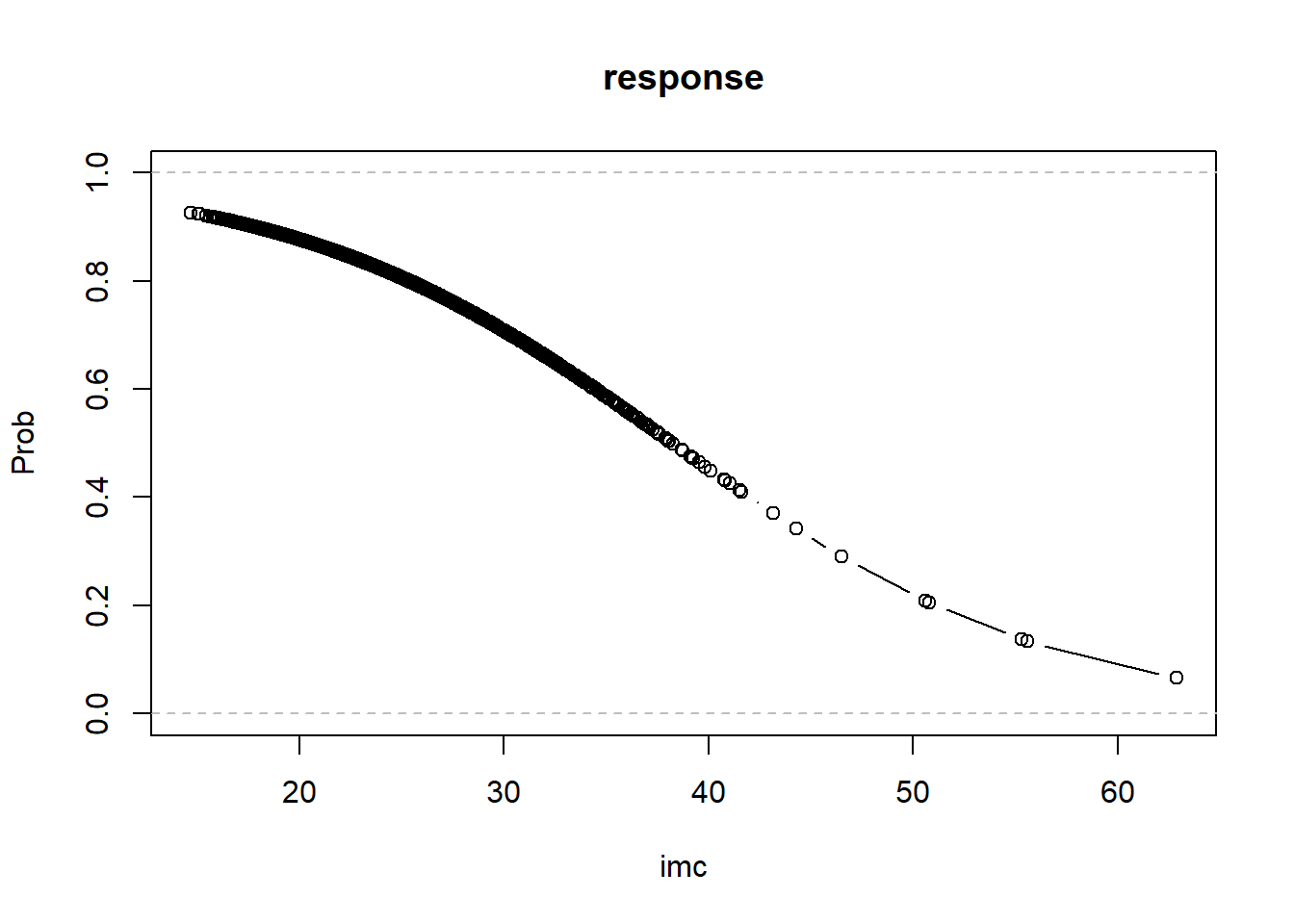 If we have two covariates \(x_1\) and \(x_2\), then the logistic regression model is:
\[log(odds)=\beta_0+\beta_1x_1+\beta_2x_2 \quad \Rightarrow \quad odds=e^\beta_0\times e^{\beta_1x_1}\times e^{\beta_2x_2}\]
Now \(\beta_1\) can be interpreted as follows: a unit increase in \(x_1\) with \(x_2\) held fixed, increases
the log-odds of the response by \(\beta_1\) or increases the odds of the response by a factor of \(e^\beta_1\).
Let’s look at the case when one variable is continuous and the other is categorical, for that we will use the predictors sex and age. We first consider the case in which there is no interaction between them:
# Obtain fitted probabilities
lmod.sexage=glm(g02 ~ sex+age, family = binomial, health)
summary(lmod.sexage)
##
## Call:
## glm(formula = g02 ~ sex + age, family = binomial, data = health)
##
## Coefficients:
##              Estimate Std. Error z value Pr(>|z|)
## (Intercept)  3.797233   0.120809  31.432  < 2e-16 ***
## sex2        -0.395887   0.061899  -6.396  1.6e-10 ***
## age         -0.051446   0.002512 -20.478  < 2e-16 ***
## ---
## Signif. codes:  0 '***' 0.001 '**' 0.01 '*' 0.05 '.' 0.1 ' ' 1
##
## (Dispersion parameter for binomial family taken to be 1)
##
##     Null deviance: 7177.9  on 7356  degrees of freedom
## Residual deviance: 6685.8  on 7354  degrees of freedom
## AIC: 6691.8
##
## Number of Fisher Scoring iterations: 4
So, on the scale of the linear predictor we are fitting two parallel lines, that is, we assume that the rate of change of the logit as age increases is the same for males and females
par(mfrow=c(1,2))
# Obtain fitted linear predictor
fittedlp=predict(lmod.sexage)
#Plot linear predictor for males and females
plot(health$age,fittedlp,type="n",main="No interaction (logit)",
xlab="Age",ylab="Linear predictor")
#Get ages and linear predictor for males
age1=health$age[health$sex==1]
lp1=fittedlp[health$sex==1]
#Order according to age
o=order(age1)
lines(age1[o],lp1[o],col=2,t='l')
#Get ages and linear predcitor for females
age2=health$age[health$sex==2]
lp2=fittedlp[health$sex==2]
#Order according to age
o=order(age2)
lines(age2[o],lp2[o],col=4,t='l')
legend(15,1, col=c(2,4),c("male","female"),lty=1,bty="n",cex=0.8)
#Repeat the plot for fitted probabilities
# Obtain fitted linear probabilities
fittedp=predict(lmod.sexage, type="response")
#Plot probailities for males and females
plot(health$age,fittedp,type="n",main="No interaction (prob.)",xlab="Age",
ylab="Probability")
#Get ages and probabilities for males
age2=health$age[health$sex==1]
p1=fittedp[health$sex==1]
#Order according to age
o=order(age1)
lines(age1[o],p1[o],col=2,t='l')
#Get ages and probabilities for females
age2=health$age[health$sex==2]
p2=fittedp[health$sex==2]
#Order according to age
o=order(age2)
lines(age2[o],p2[o],col=4,t='l')
legend(15,0.65, col=c(2,4),c("male","female"), lty=1, bty="n",cex=0.8)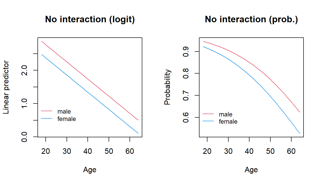 Now, we include the interaction between
 age and sex, and so, the rate of change can be different for each gender:
We can plot the estimated probabilities from model lmod.imc
# Obtain fitted probabilities
lmod.sexage2=glm(g02 ~ sex+age+sex:age, family = binomial, health)
summary(lmod.sexage2)
##
## Call:
## glm(formula = g02 ~ sex + age + sex:age, family = binomial, data = health)
##
## Coefficients:
##              Estimate Std. Error z value Pr(>|z|)
## (Intercept)  3.653489   0.170571  21.419   <2e-16 ***
## sex2        -0.135450   0.230287  -0.588    0.556
## age         -0.048200   0.003721 -12.952   <2e-16 ***
## sex2:age    -0.005918   0.005046  -1.173    0.241
## ---
## Signif. codes:  0 '***' 0.001 '**' 0.01 '*' 0.05 '.' 0.1 ' ' 1
##
## (Dispersion parameter for binomial family taken to be 1)
##
##     Null deviance: 7177.9  on 7356  degrees of freedom
## Residual deviance: 6684.4  on 7353  degrees of freedom
## AIC: 6692.4
##
## Number of Fisher Scoring iterations: 4
The estimated parameter for the interaction seems quite small compared with the parameter for sex, so probably both rates of change will continue to be very similar. We can see this graphically:
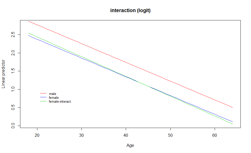 The linear predictor for females when an interaction term is included in the model is almost identical to the one without interction.
When there exists an interaction between a factor and a continuous variable the estimated parameter for the factor depends on the variable that interacts with it. We cannot obtain the odds-ratio (OR) by taking exponentials
To obtain the ORs in the presence of interaction:
- Write the equation of the logit for both levels of the risk factor
- Compute the difference between the logits
- Take the exponential of the obtained difference
Consider a model with 2 variables and their interaction. Let us say, a factor \(F\) and a continuous predictor \(X\) and \(F \times X\). The logit for \(F = f\) and \(X = x\) is: \[ log \left ( \frac{p(f,x)}{1-p(f,x)}\right )=\beta_0+\beta_1f+\beta_2x+\beta_3f\times x, \] Suppose that we want to calculate the OR between the two levels of \(F\), \(f_1\) versus \(f_0\): \[\begin{aligned} log \left ( \frac{p(f_1,x)}{1-p(f_1,x)}\right )=&\beta_0+\beta_1f_1+\beta_2x+\beta_3f_1\times x\\ log \left ( \frac{p(f_0,x)}{1-p(f_0,x)}\right )=&\beta_0+\beta_1f_0+\beta_2x+\beta_3f_0\times x\\ log \left ( \frac{p(f_1,x)}{1-p(f_1,x)}\right )- log \left ( \frac{p(f_0,x)}{1-p(f_0,x)}\right )=&\beta_1(f_1-f_0)+\beta_3x(f_1-f_0)\\ OR=&exp\left [ \beta_1(f_1-f_0)+\beta_3x(f_1-f_0)\right ] \end{aligned}\] In our health perception example, we have:
##  (Intercept)         sex2          age     sex2:age
##  3.653488923 -0.135449547 -0.048200283 -0.005918381
For the comparison between females and males: \[OR = exp(-0.124-0.006\times age)\]
Exercise 13
Fit a logistic regression model to predict the probability self-perceived health using the predictors sex and weight without including the interaction between them.
- Interpret the coefficients in terms of odds ratios
- Plot the predicted probabilities for males and females
- Given that a person has \(weight=95\), what is the relative risk and odds ratio of self-perceived good health of a female compared with a male?
- Repeat the analysis including the interaction between
weightandsexin the model, and compare and comment the results
6.5 Parameter Inference
Statistical inference in logistic regression is based on certain properties of maximum likelihood estimators and on likelihood ratio tests
Wald test
It is based on the asymptotic distribution of the maximum likelihood estimators: \[\boldsymbol{\hat \beta}\approx N\left ( \boldsymbol{\beta}, Var(\boldsymbol{\hat \beta}) \right ),\]
and \(Var(\boldsymbol{\hat \beta})\) is the inverse of the information matrix \(I(\boldsymbol{\beta})=-E \left [\frac{\partial^2 \ell (\boldsymbol{\beta})}{\partial \boldsymbol{\beta}\partial \boldsymbol{\beta}^\prime} \right ]\). In order to test whether a coefficient is zero: \[H_0: \beta_j=0\quad Z_0=\frac{\hat \beta_j}{\sqrt{Var(\hat \beta_j)}}\] The test statistic \(Z_0\) follows an asymptotic standard-normal distribution, and we can calculate the p-value under the null hypothesis. Similarly, an asymptotic \((1-\alpha)\%\) confidence interval for is given by \[\hat \beta_j\pm z_{\alpha/2}S.E.(\hat \beta_j)\] If we call L the minimun of that interval and U the maximum, then, a confidence interval for the odds ratio is given by \((e^L, e^U)\)
In R this is the test carried out in the output of the glm() function:
The estimated coefficients for sex and age and their interaction in model lmod.sexage2 are:
##
## Call:
## glm(formula = g02 ~ sex + age + sex:age, family = binomial, data = health)
##
## Coefficients:
##              Estimate Std. Error z value Pr(>|z|)
## (Intercept)  3.653489   0.170571  21.419   <2e-16 ***
## sex2        -0.135450   0.230287  -0.588    0.556
## age         -0.048200   0.003721 -12.952   <2e-16 ***
## sex2:age    -0.005918   0.005046  -1.173    0.241
## ---
## Signif. codes:  0 '***' 0.001 '**' 0.01 '*' 0.05 '.' 0.1 ' ' 1
##
## (Dispersion parameter for binomial family taken to be 1)
##
##     Null deviance: 7177.9  on 7356  degrees of freedom
## Residual deviance: 6684.4  on 7353  degrees of freedom
## AIC: 6692.4
##
## Number of Fisher Scoring iterations: 4## Waiting for profiling to be done...## 2.5 % 97.5 %
## (Intercept) 3.32361013 3.99253507
## sex2 -0.58784069 0.31521457
## age -0.05554669 -0.04095319
## sex2:age -0.01580544 0.00397876## Waiting for profiling to be done...## 2.5 % 97.5 %
## (Intercept) 27.7603884 54.1920962
## sex2 0.5555255 1.3705534
## age 0.9459679 0.9598741
## sex2:age 0.9843188 1.0039867As it could be expected that the interaction is not is not a significant, i.e. the effect of age on self-perceived health is similar for males and females.
Using the relationship between the odds and the probability we can get confidence intervals for the estimated probabilities \[ \frac{e^{I.C. logit}}{1+ e^{I.C. logit}}\]
#Get fitted values of logit and their standard errord
fitted=predict(lmod.sexage, se.fit=TRUE)
names(fitted)
#Calculate lower limit of C.I. for probability by transforming lower limit of C.I. of logit
L.inf=with(fitted,exp(fit-1.96*se.fit)/(1+exp(fit-1.96*se.fit)))
L.sup=with(fitted,exp(fit+1.96*se.fit)/(1+exp(fit+1.96*se.fit)))
with(fitted,plot(health$age[health$sex==1],(exp(fit)/(1+exp(fit)))[health$sex==1],
                 ylim=c(0.1,1),ylab="Probability",xlab="Age",pch=19,cex=0.5))

points(health$age[health$sex==1],L.inf[health$sex==1],col=2,pch=19,cex=0.5)
points(health$age[health$sex==1],L.sup[health$sex==1],col=2,pch=19,cex=0.5)
legend(20,0.6, c("Probability","C.I."),col=c(1,2),pch=c(19,19),bty="n",cex=c(0.9,0.9))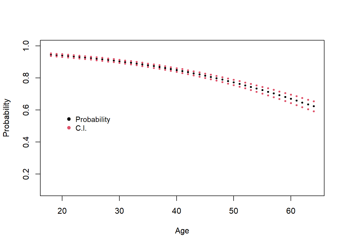
Exercise 14
- Calculate and interpret the confidence intervals for the coefficients in the model fitted the previous exercise (including the interaction)
- Calculate the estimated expected probability of males of 80 and 165 kg and give a confidence interval for each of those predictions
6.6 Variable selection
As in the case of linear regression, we can select the variable in our model using a test-based procedure or an criterion-based procedure
Likelihood Ratio Test
A likelihood ratio test can be used to compare a full model with a reduced model that is of interest. This is analogous to the extra-sum-of-squares in the Analysis of Variance that we have used previously to compare full and reduced models.
The saturated model is the model that has as many parameters as data values, i.e. \(\hat y_i=y_i\). Then, the comparison between the observed values and the fitted values is done with the Deviance (\(D\)); \[D=-2\log\underbrace{\left [ \frac{\text{likelihood of the fitted model}}{\text{likelihood of the saturated model}}\right]}_{(*)}\] The value \((*)\) is called Likelihood ratio. We take logarithm and multiply by 2 to obtain that \(D\sim \chi^2\). Since the distribution of the deviance is known, we can use it to compare nested models.
The likelihood ratio test procedure compares twice the logarithm of the value of the likelihood function for the full model (FM) to twice the logarithm of the value of the likelihood function of the reduced model (RM) to obtain a test statistic: \[LRT=D(RM)-D(FM)= -2log \left ( \frac{\mathcal{L}(RM)}{\mathcal{L}(FM)}\right )=2[log (\mathcal{L}(FM))-log(\mathcal{L}(RM)]\sim \chi^2_{k-q}\]
Under the null hypothesis, this test statistic has an asymptotic chi-square distribution with degrees of freedom equal to the difference in the number of parameters between the full, \(k\), and reduced, \(q\), models.
# Logistic Regression using sex and age and the interaction
summary(lmod.sexage2)
##
## Call:
## glm(formula = g02 ~ sex + age + sex:age, family = binomial, data = health)
##
## Coefficients:
##              Estimate Std. Error z value Pr(>|z|)
## (Intercept)  3.653489   0.170571  21.419   <2e-16 ***
## sex2        -0.135450   0.230287  -0.588    0.556
## age         -0.048200   0.003721 -12.952   <2e-16 ***
## sex2:age    -0.005918   0.005046  -1.173    0.241
## ---
## Signif. codes:  0 '***' 0.001 '**' 0.01 '*' 0.05 '.' 0.1 ' ' 1
##
## (Dispersion parameter for binomial family taken to be 1)
##
##     Null deviance: 7177.9  on 7356  degrees of freedom
## Residual deviance: 6684.4  on 7353  degrees of freedom
## AIC: 6692.4
##
## Number of Fisher Scoring iterations: 4
The output of summary() returns, the residual deviance and the null deviance. The deviance correspond to de deviance of the model fitted and the null deviance correspond to a model in wich only the constant is fitted. We could use this information to carry out a test similar to the F-test in linear regression (testing if all coefficients are zero):
# Calculate the change in deviance
7177.9-6684.4
## [1] 493.5
#Calculate the change in degrees of freedom
7356-7353
## [1] 3
# Calculate the p-value
1-pchisq(493.5,3)
## [1] 0
The test based on the change in deviance can also be used to test for individual parameters, for example in our case study we can test whether the interaction is significant calculating the change in deviance between the model with and without interaction. We can use the function anova() to do so:
#use function anova, now we need to specify the distribution of the test
anova(lmod.sexage2,lmod.sexage, test="Chisq")
## Analysis of Deviance Table
##
## Model 1: g02 ~ sex + age + sex:age
## Model 2: g02 ~ sex + age
##   Resid. Df Resid. Dev Df Deviance Pr(>Chi)
## 1      7353     6684.4
## 2      7354     6685.8 -1  -1.3746    0.241
In practice, you should always test for the sigfinicance of the interaction before testing for the significance of the individual terms.
Wald versus likelihood (deviance) ratio test
The likelihood ratio test provides the asymptotically more powerful and reliable test. The likelihood ratio test is almost always preferable to the Wald test
Akaike Informatin Criteria, Bayesian Information Criteria
The Akaike Information Criterion (AIC) provides a method for assessing the quality of your model through comparison of related models. It’s based on the Deviance, but penalizes you for making the model more complicated. Much like adjusted R-squared, it’s intent is to prevent you from including irrelevant predictors.
However, unlike adjusted R-squared, the number itself is not meaningful. If you have more than one similar candidate models (where all of the variables of the simpler model occur in the more complex models), then you should select the model that has the smallest AIC.
\[AIC= 2\times Deviance+ 2\times q \quad BIC= 2\times Deviance+ log(n)\times q,\] where \(q\) is the number of parameters in the model.
Let’s compare model lmod.sexageand lmod.sexage2 using AIC and BIC
## [1] 6691.787## [1] 6692.413#We can calculate BIC using the deviance
2*summary(lmod.sexage)$deviance+log(nrow(health))*length(coef(lmod.sexage))## [1] 13398.28## [1] 13404.44Using both criteria, the best model is the one without the interaction. The function stepAIC can be use to sellect the best model using either of these two criteria
6.7 Model diagnostics
When the hypothesis of the logistic regression model are violated, the fitted model can give the next kind of errors:
- Biased coefficients (systematic tendency of over/under estimate the coefficients of the model.)
- Unefficient estimators (large standard errors for the coefficient’s estimates)
- Statistical Inference on the parameters is not valid
- Other issues: high-leverage points of the predictors or outliers in the response, that may affect the estimation of the parameters.
We will focus on the hypotheses of the model and how to detect when they are violated
Specification error
To check if the model is well specified. We need to study:
- The functional relationship between the predictors and the response.
- The presence of irrelevant predictors and the absence of important variables.
If the model is not correctly specified (possible causes):
- The relation of the logit and the predictors is not linear.
- The relation between the variables is multiplicative, not additive (there is interaction).
- There are more variables than needed (the standard errors of the estimated coefficients increases, the eficiency of the estimadors are reduced, although there is no bias).
- Presence of multicolinearity, i.e. correlated predictors.
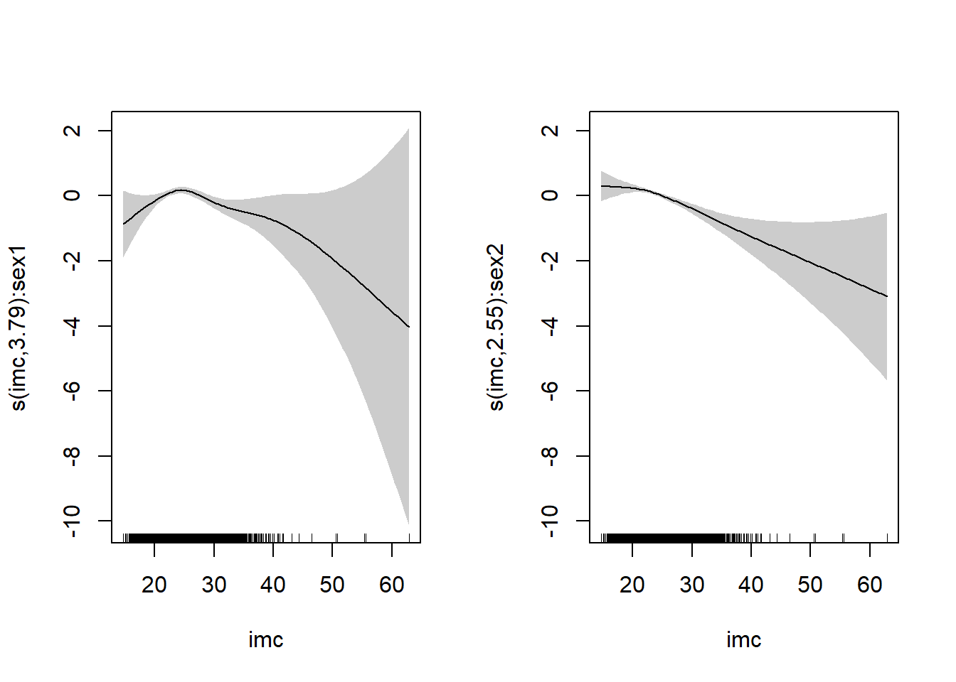
If the relationship between the logit and the predictors is not linear, a unit
increment of \(X\) is not constant, and do depends on the value of \(X\). We can detect the non-linearity using a smoothing technique and the
function gam() in the package mgcv (we will see this at the end of the course)
 Residual analysis
In the case of GLMs, there are also several type of residuals that we can define:
Response residuals: \(y_i-\hat \mu_i\), they are not appropriate since \(Var(y_i)\) is not constant.
Pearson residuals: They have constant variance and mean zero. Mostly useful for detecting variance misspecification \[ r_{i,P}=\frac{y_i-\hat \mu_i}{\sqrt{\widehat{Var(y_i)}}} \]
Deviance residuals: \[ sign(y_i-\hat \mu_i)\sqrt{d_i^2} \] where \(d_i\) is the contribution to the model deviance of the ith observation. For many models the deviance residuals are closer to a Normal distribution than the Pearson residuals, and so they are more appropriate for constructing diagnostic plots.
Standardized residuals: Both the Pearson and the deviance residuals can be variance-standardized and corrected for the efects of leverage by dividing them by \(\sqrt{1-h_{ii}}\). These residuals should lie within \(-2\) and \(+2\).
We should make the following plots:
- For checking the systematic part of the model, one can plot residuals
against the predicted values (either the linear predictor or the
probabilities). In the binary data case where we obtain two curves, one
corresponding to residuals for the
1-observations and another for the0-observations, this pattern is due to the binary nature of the response and that not indicate a bad fit, in this case for an acceptable fit one would expect that locally the residuals average to zero). - Plot absolute values of residuals against fitted values, an ill chosen variance function will result in a trend in the mean.
The function glm.diag.plots() in the package boot
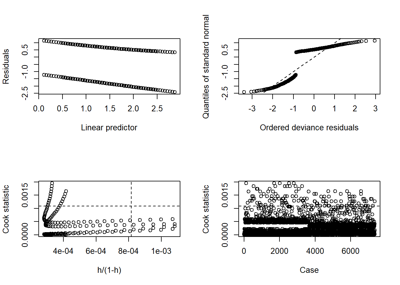
In the case of binary data, the qqplot does not make sense. The plot of the Cook’s distance is similar to the one in linear regression, so the problematic points are the ones above the horizontal and to the right of the vertical lines.
In this case is better to use \(r_Q\) (package statmod)
 library(statmod)
par(mfrow=c(1,2))
plot(health$age,qres.binom(lmod.sexage), xlab="Age",ylab="Quantile residuals")
qqnorm(qres.binom(lmod.sexage))
abline(a=0,b=1,col="red")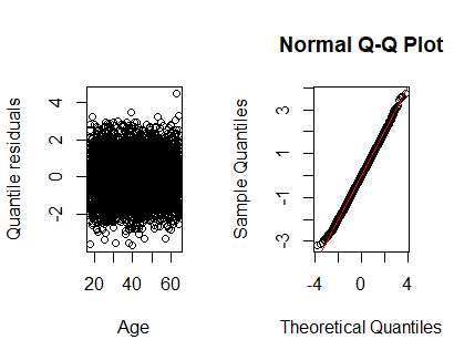
6.7.1 Goodness of fit
An important question in any regression analysis is whether the proposed model
adequately fits the data, which leads naturally to the notion of a formal test for
lack-of-fit (or goodness of fit). In other examples of GLMs, the deviance is a measure of how well the model fit
the data, but in the case of binary data it cannot be used. As an alternative
the Hosmer-Lemeshow test (Hosmer and Lemeshow 1980). The aim of the test is to check if the proposed model can explain what is observed, i.e., we evaluate the distance between the observed and what is expected, and it is a version of the pearson’s X\(^2\) test. In this test the null hypothesis is that the fitted model is correct. The test available in the package ResourceSelection using the function hoslem.test(). The arguments are: the response (given as 0s and 1s) and the predicted probabilities.
In our case study let’s fit the following model:
##
##  Hosmer and Lemeshow goodness of fit (GOF) test
##
## data:  health$g02, predict(lmod.sexage, type = "response")
## X-squared = 12.729, df = 8, p-value = 0.1215
The p-value of indicates that the Goodness of Fit is ok (a large p-value indicates no evidence of poor fit)
Exercise 15
- Use all predictors available in the dataset
healthto find the best subset of predictors (and their possible interactions) using LRT, AIC and BIC - Are the chosen models the same?. If the answer is not, which one would you use as your final model?
- Use the Hosmer-Lemeshow test to check the goodness of fit of the model obtained
6.8 Validation of predicted probabilities
The logistic regression predicts the logit of an event outcome from a set of predictors. Since the logit it the log of the odds, we can always transform back to the probability scale. The predicted probabilities can be revalidated with the actual outcome to check if high probabilities are associated with events and low probabilities with non-events. The degree to which predicted probabilities agree with the outcomes maybe expressed as a classification table or as a measure of association.
6.8.1 Classification table or contingency table
Given that we estimate probabilities for individuals, how can we translate this into a predicted outcome? Two possibilities for prediction rules are:
- Use 0.5 as a cutoff. That is, if the predicted probability is greater than 0.5, its predicted
outcome is 1, otherwise is 0. This approach is reasonable when:
- It is equally likely in the population of interest that an outcome 0 or 1 occur.
- The cost of incorrectly 0 and 1 are approximately the same.
- Find the best cutoff for the data set. Using this approach, we evaluate different cutoffs
values and calculate for each of them the proportion of observation incorrectly classified.
Then, we select the cutoff that minimized the proportion of misclassified observations.
This approach is reasonable when:
- The data set is a random sample from the population of interest.
- The cost of incorrectly 0 and 1 are approximately the same.
We create the following classification table, where \(\hat y_i=1\) if \(\hat p_i > s\) (where \(s\) is a given cutoff point):
| \(y=1\) | \(y=0\) | Total | |
|---|---|---|---|
| \(\hat y=1\) | a | b | a+b |
| \(\hat y=0\) | c | d | c+d |
| Total | a+c | b+d |
Then, we define:
- Sensitivity: the proportion of true positives or the proportion of true 1s estimated as 1s \(a/(a+c)\)
- Specificity: the proportion of true negatives or the proportion of 0s estimated as 0s, \(d/(b+d)\)
- False positive rate: the proportion of true 0s estimated as 1s, \(b/(b+d)\)
- False negative rate: the proportion of true 1s estimated as 0s, \(c/(a+c)\)
Our aim will be to find the cutoff that maximizes the sensitvity and specificity
6.8.2 ROC curve
The ROC (Receiver Operating Characteristic) curve is a graphic display that gives a measure of the predictive accuracy of the model. It allows to represent the impact of the cutoff point on the sensitivity and specificity (keep in mind that as you increase the cutoff point from 0 to 1, the sensitivity decreases and the specificity increases). Ideally, we would like to have high values for both sensitivity and specificity.
The ROC curve is a plot of Sensitivity against 1-Specificity (False positive rate) for all cutoff points. Then, area under the curve (AUC) is computed. For a model with high predictive accuracy, the ROC curve rises quickly. The AUC takes values between 0 and 1. The larger the AUC, the better the hability of the model to discriminate between individuals that presents the response of interest and who don’t.
In general
AUC \(\leq 0.6\): the model is worthless, it does not help us to discriminate
\(0.6\leq AUC \lt 0.8\): acceptable
\(0.8\leq AUC \lt 0.9\): good
\(AUC\geq 0.94\): outstanding
We use the ROC() function in the package Epi.
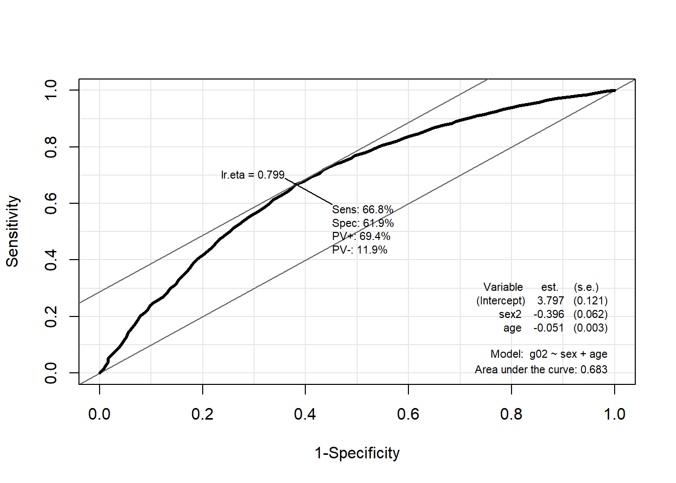 The optimal cutoff is 0.7899 and the model is only acceptable in terms of predicting power
Exercise 16
Calculate the AUC and optimal cutoff point for the model obtained in the previous exercise
6.9 Logistic regression for grouped data
Sometimes, the data are grouped with respect to the value of the
covariates that they share. For example, suppose we ask 7
individuals whether they use the public transport or not (the
response) and we use two explanatory variables: \(x_1=1,2\), takes
the value 1 if the individual is under 21 years of age and value two
otherwise. The variable \(x_2=1,2\), takes value 1 if there is a car
if the household and 2 otherwise. We could represent the data in two
different ways:
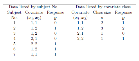 When binary data are grouped by covariate class, the responses have
the form \(y_i/n_i\), where \(0\leq y_i\leq n_i\) is the number of
successes out of the \(n_i\) individuals in the \(ith\) covariate class,
and the total number of individuals is \(n=\sum_{i=1}^g n_i\). If data are
ungrouped, there are as many covariate classes as individuals and
\(n_i=1\). In this context arises the binomial distribution.
\[f(Y_i)=\binom{n_i}{y_i}p_i^{y_i} (1-p_i)^{n_i-y_i} \quad i=1, \ldots , g\]
Estimation would be done also using maximum likelihood and inference on the estimated coefficients woul carry out in a similar way. H+owever, there are some aspects that are different:
- Goodness of fit test: Now we can use the deviance as a goodness of fit measure of the model (no need for the Hosmer-Lemeshow test): \[D\sim \chi^2_{n-k-1}\]
- Binomial data are asymptotically Normal, therefore, if we have grouped data, we can use a q-q normal plot of deviance residuals to check that the assumption of distribution is correct
To fit logistic regression for grouped data in R, we use the glm() function but we need to included the values of \(Y_i\) and \(n_i\), we can do this in two differen ways:
- The response is a matrix with two columnuns , each row is giben by \((y_i,n_i)\)
- The response is the proportion \(y_i/n_i\) and we include the argument
weightsequal to \(n_i\).
6.9.1 Case study: The Flight of the Space Shuttle Challenger

On January 28, 1986, the space shuttle Challenger took off on the 25th flight in NASA’s space shuttle program. Less than 2 minutes into the flight, the spacecraft exploded, killing all on board. A Presidential Commission was formed to explore the reasons for this disaster.
First, a little background information: the space shuttle uses two booster rockets to help lift it into orbit. Each booster rocket consists of several pieces whose joints are sealed with rubber O-rings, which are designed to prevent the release of hot gases produced during combustion. Each booster contains 3 primary O-rings (for a total of 6 for the orbiter). In the 23 previous flights for which there were data, the O-rings were examined for damage.
One interesting question is the relationship of O-ring damage to temperature (particularly since it was
(forecasted to be) cold, \(31^o\) F, on the morning of January 28, 1986). There was a good deal of discussion
among the engineers the previous day as to whether the
flight should go on as planned or
not (an important point is that no data scientist were involved in the discussions). But they only look at the temperature of the days in which there was O-ring damage
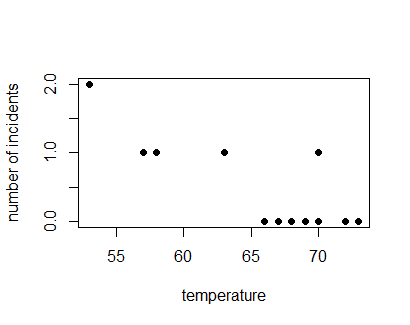 This was a mistake, since most of the cases in which there were no failures occured with higher temperatures. The decision they took was to allow the launch of the spaceship with catastrophic results. Now we will carry out the analysis as it should have been done. The dataset
 challenger.txt has data on temperature, the number of O-rings damaged and the number of O-rings in the spaceship.
## [1] "Temp" "Damaged" "O.rings"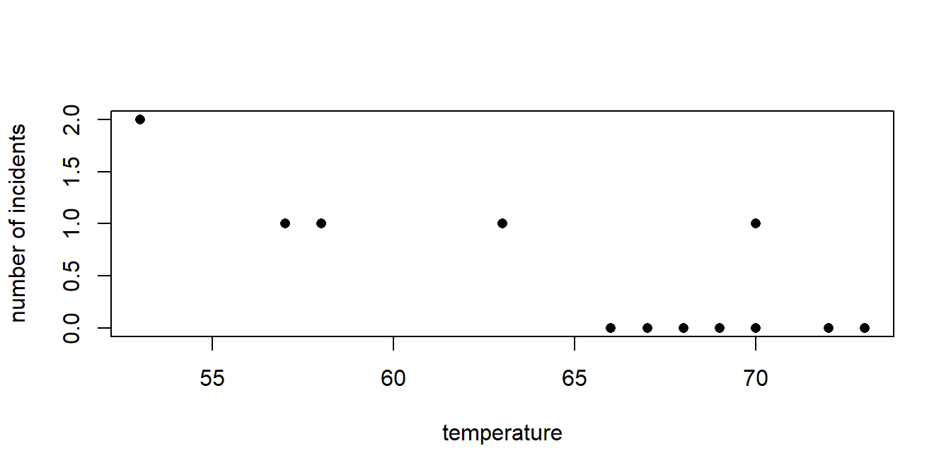 Let’s fit a logistic regression model to check the impact of temperature on the probability of failure
orings.mod=glm(Damaged/O.rings~Temp, family=binomial, weights=O.rings,data=orings)
summary(orings.mod)
##
## Call:
## glm(formula = Damaged/O.rings ~ Temp, family = binomial, data = orings,
## weights = O.rings)
##
## Coefficients:
## Estimate Std. Error z value Pr(>|z|)
## (Intercept) 7.71743 3.91782 1.970 0.0489 *
## Temp -0.16066 0.06347 -2.531 0.0114 *
## ---
## Signif. codes: 0 '***' 0.001 '**' 0.01 '*' 0.05 '.' 0.1 ' ' 1
##
## (Dispersion parameter for binomial family taken to be 1)
##
## Null deviance: 15.4630 on 15 degrees of freedom
## Residual deviance: 8.8415 on 14 degrees of freedom
## AIC: 24.18
##
## Number of Fisher Scoring iterations: 5Exercise 17
Using the previous model:
- Plot the predicted probabilities for 100 different values of temperature between \(20\) and \(80\) degrees Fahrenheit
- Estimate the odds ratio for O-ring failure with a 10 degree decrease in the launch temperature.
- The launch temperature that day was 31 degrees. Based on data from the first 23 launches, estimate the probability of a O-ring failure on the Challenger flight. -Provide a confidence interval for that probability. What would you have done if you had to make the decision?, Why?.
6.10 Further exercises in logistic regression
Exercise 18
In a study on infant respiratory disease, data are collected on a sample of 2074 infants. The information collected includes whether or not each infant developed a respiratory disease in the first year of their life; the gender of each infant; and details on how they were fed as one of three categories (breast-fed, bottle-fed and supplement). The data are tabulated in R as follows:
   disease nondisease gender food
1      77        381    Boy Bottle-fed
2      19        128    Boy Supplement
3      47        447    Boy Breast-fed
4      48        336   Girl Bottle-fed
5      16        111   Girl Supplement
6      31        433   Girl Breast-fed
We fit the following model:
> total <- disease + nondisease
> model1 <- glm(disease/total ~ gender + food, family = binomial,
+ weights = total)
> summary(model1)
Coefficients:
Estimate Std. Error z value Pr(>|z|)
(Intercept)    -1.6127     0.1124  -14.34 < 2e-16 ***
genderGirl     -0.3126     0.1410  -2.216 0.0267 *
foodBreast-fed -0.6693     0.1530  -4.374 1.22e-05 ***
foodSupplement -0.1725     0.2056  -0.839 0.4013
---
Null deviance: 26.37529 on 5 degrees of freedom
Residual deviance: 0.72192 on 2 degrees of freedom
Write the equation for model1
What would be the probability that a girl bottle-fed has a respiratory disease
Calculate a \(95\%\) confidence intervals for the odds ratio of having the disease of girls who were breasted-fed versus girls who were bottled-fed
Explain which hypothesis tests are being carried out in the following output:
 > anova (model1,test="Chisq")
 Analysis of Deviance Table
 Df Deviance Resid. Df Resid. Dev  Pr(>Chi)
 NULL                     5    26.3753
 sex   1   5.4761         4    20.8992   0.01928 *
 food  2  20.1772         2     0.7219 4.155e-05 ***
Why would not make sense to fit the following model:
 model2 <- glm(disease/total ~ gender + food + gender:food,
  family = binomial, weights = total)
Exercise 19
Results from a Copenhagen housing condition survey are compiled in an R data frame housing1 consisting of the following components:
- {Infl: Influence of renters on management: Low, Medium, High
- Type: Type of rental property: Tower, Atrium, Apartment, Terrace.
- Cont: Contact between renters: Low, High.
- Sat: Highly satisfied or not: two columns of counts.
A model is fitted to the data using the following commands.
fit <- glm(Sat~Infl+Type+Cont,family=binomial,data=housing1) Part of the results are summarized below:
Coefficients:

Estimate Std. Error z value Pr(>|z|)
(Intercept)   -0.6551     0.1374  -4.768 1.86e-06 ***
InflMedium     0.5362     0.1213   4.421 9.81e-06 ***
InflHigh       1.3039     0.1387   9.401 < 2e-16 ***
TypeApartment -0.5285     0.1295  -4.081 4.49e-05 ***
TypeAtrium    -0.4872     0.1728  -2.820 0.00480 **
TypeTerrace   -1.1107     0.1765  -6.294 3.10e-10 ***
ContHigh       0.3130     0.1077   2.905 0.00367 **

(Dispersion parameter for binomial family taken to be 1)

Null deviance: 166.179 on 23 degrees of freedom
Residual deviance: 27.294 on 17 degrees of freedom
AIC: 146.55- Write the equation of the fitted model
- According to the fitted model, what percentage of renters, who have low influence on management, live in apartment, and have high contact between neighbors, are highly satisfied?
- Do people who live in apartments have a significantly different probability of satisfaction than people who live in atriums? The correlation between the respective coefficients is 0.494.
- Estimate the odds ratio of high satisfaction for groups with high contact among neighbors over groups with low contact among neighbors, using a 95\(\%\) confidence interval.