Chapter 3 Multiple Linear Regression II: Model selection and diagnostics
The process for choosing a model involves several procedures (variable selection, verifying assumptions, variable transformation, etc.), but the order of the procedures is not always the same, and the analyst should be alert for unspected structure in the data.
3.1 Model selection
Building a model implies looking for the best subset of predictors that explains the data in the simplest way, since adding too many predictors will add unwanted noise to the problem and will probably invalid the explanatory purpose of the model.
There are two main approaches:
- Stepwise testing strategy
- Criterion approach that attemps to maximize some measure of goodness of fit
3.1.1 Testing-based procedures
These methods are easy to implement. However, the final model can be too parsimoniuos (too simple) and the analyst may want to include predictors that appear to have no statistical significance but may have scientific significance.
1. Backwards elimination
- Begin with a model that contains all possible preditors
- Identify the predictor with the largest p-value. This can be done looking at the ouput of
summaryor using thedrop1()function - If the p-value is greater than a pre-specified value \(\alpha_{crit}\) (0.15 or 0.2), drop the variable
- Repeat the process until the p-value of the remaining variables are bellow \(\alpha_{crit}\)
2. Forward selection
- Begin with no pedictors
- Include the predictor with the smallest p-value bellow the \(\alpha_{crit}\) when included in the model. This can be done looking at the ouput of
summaryor using theadd1function - Repeat the process until no new predictors can be added
3. Stepwise regression
- It is a combination of the previous two methods
- Variables that were removed or added in a previus step can reenter or exit the model later in the process
3.1.2 Criterion-based procedures
There several optimality criteria used in a model building process, we will focus con two of them: \(R^2_a\) (previuosly introduced) and Akaike Information Criterion (\(AIC\),Akaike (1973)). Given a model \(M\), the AIC criterion is defined as: \[AIC(M)=-2 max(ln(L(\sigma^2,\mathbf{\beta}|\mathbf{X})))+2\times e.d(M)+constant=2ln(SSE/n)+ 2\times e.d(M)+constant\] \(AIC\) is a trade-off between a model with fitted values close to the data (small \(SSE\)), and a model with few parameters (small \(e.d.\)). And we will look for the model that minimizes the \(AIC\) criterion.
AIC:
- Is not a measure of the goodness of fit of the model
- It does not say anything about the predicte power of the model
- We will see later in the course cross-validation (\(CV\)) which is an estimate of predictive power
3.1.3 Case study application
We will search for the best subset of predictors using the backwards procedure and \(\alpha_{crit}=0.2\)
Let’s illustrate it using the case study. Recall
# Model with all predictors
modall <- lm(hwfat ~., data = bodyfat)
summary(modall)$coefficients
##                Estimate Std. Error    t value     Pr(>|t|)
## (Intercept) 13.29369860 9.63026704  1.3804081 1.717917e-01
## age         -0.32893403 0.32157778 -1.0228755 3.098393e-01
## ht          -0.06730905 0.16050751 -0.4193514 6.762255e-01
## wt          -0.01365183 0.02590783 -0.5269385 5.998789e-01
## abs          0.37141976 0.08836595  4.2032001 7.548985e-05
## triceps      0.38742647 0.13761017  2.8153912 6.301113e-03
## subscap      0.11405213 0.14192779  0.8035927 4.243145e-01
drop1(modall,test="F")
## Single term deletions
##
## Model:
## hwfat ~ age + ht + wt + abs + triceps + subscap
##         Df Sum of Sq    RSS    AIC F value    Pr(>F)
## <none>               651.05 179.51
## age      1     9.594 660.64 178.65  1.0463  0.309839
## ht       1     1.613 652.66 177.70  0.1759  0.676225
## wt       1     2.546 653.60 177.81  0.2777  0.599879
## abs      1   162.000 813.05 194.84 17.6669 7.549e-05 ***
## triceps  1    72.683 723.73 185.76  7.9264  0.006301 **
## subscap  1     5.921 656.97 178.21  0.6458  0.424315
## ---
## Signif. codes:  0 '***' 0.001 '**' 0.01 '*' 0.05 '.' 0.1 ' ' 1
The largest p-value, \(0.676\) corresponds to ht, so, we drop it
# Model without ht
mod1=update(modall,.~.-ht)
drop1(mod1,test="F")
## Single term deletions
##
## Model:
## hwfat ~ age + wt + abs + triceps + subscap
##         Df Sum of Sq    RSS    AIC F value    Pr(>F)
## <none>               652.66 177.70
## age      1     9.875 662.54 176.87  1.0894  0.300098
## wt       1    10.554 663.22 176.95  1.1643  0.284169
## abs      1   189.072 841.73 195.54 20.8580 1.996e-05 ***
## triceps  1    78.809 731.47 184.59  8.6941  0.004302 **
## subscap  1     5.693 658.36 176.38  0.6281  0.430660
## ---
## Signif. codes:  0 '***' 0.001 '**' 0.01 '*' 0.05 '.' 0.1 ' ' 1
The largest p-value, \(0.4306\) corresponds to subscap
# Model without subscap
mod2=update(mod1,.~.-subscap)
drop1(mod2,test="F")
## Single term deletions
##
## Model:
## hwfat ~ age + wt + abs + triceps
##         Df Sum of Sq    RSS    AIC F value    Pr(>F)
## <none>               658.36 176.38
## age      1    13.615 671.97 175.97  1.5097    0.2231
## wt       1     6.833 665.19 175.18  0.7577    0.3869
## abs      1   220.994 879.35 196.95 24.5043 4.621e-06 ***
## triceps  1   201.768 860.12 195.23 22.3725 1.068e-05 ***
## ---
## Signif. codes:  0 '***' 0.001 '**' 0.01 '*' 0.05 '.' 0.1 ' ' 1
Now we drop wt
# Model without wt
mod3=update(mod2,.~.-wt)
drop1(mod3,test="F")
## Single term deletions
##
## Model:
## hwfat ~ age + abs + triceps
##         Df Sum of Sq    RSS    AIC F value    Pr(>F)
## <none>               665.19 175.18
## age      1    37.595 702.78 177.47  4.1823   0.04441 *
## abs      1   282.896 948.08 200.82 31.4712 3.323e-07 ***
## triceps  1   198.891 864.08 193.59 22.1259 1.159e-05 ***
## ---
## Signif. codes:  0 '***' 0.001 '**' 0.01 '*' 0.05 '.' 0.1 ' ' 1
mod3 would give the best subset of predictors since all p-values are above 0.2
Now let’s use the forward procedure with the function add1
#Start with a model with only the intercept
mod0=lm(hwfat~1, data=bodyfat)
#The add functions includes each predictor
add1(mod0,scope=(~.+age+ht+wt+abs+triceps+subscap),test="F",data=bodyfat)
## Single term additions
##
## Model:
## hwfat ~ 1
##         Df Sum of Sq    RSS    AIC  F value    Pr(>F)
## <none>               6017.8 340.97
## age      1     175.0 5842.8 340.67   2.2765    0.1355
## ht       1     117.8 5900.0 341.43   1.5175    0.2218
## wt       1    3237.6 2780.2 282.74  88.5045 2.219e-14 ***
## abs      1    5072.8  945.0 198.57 407.9929 < 2.2e-16 ***
## triceps  1    5056.3  961.5 199.92 399.6462 < 2.2e-16 ***
## subscap  1    4939.0 1078.8 208.90 347.9456 < 2.2e-16 ***
## ---
## Signif. codes:  0 '***' 0.001 '**' 0.01 '*' 0.05 '.' 0.1 ' ' 1
The variable abs is the most significant (smallest p-value), so it is added to the model:
#Include `abs` in the model
mod1=lm(hwfat~abs, data=bodyfat)
#Use the add() function with the rest of the predcitors
add1(mod1,scope=(~.+age+ht+wt+triceps+subscap),test="F",data=bodyfat)
## Single term additions
##
## Model:
## hwfat ~ abs
##         Df Sum of Sq    RSS    AIC F value    Pr(>F)
## <none>               944.96 198.57
## age      1    80.876 864.08 193.59  7.0199 0.0098255 **
## ht       1    61.598 883.36 195.31  5.2298 0.0250250 *
## wt       1    43.734 901.22 196.87  3.6396 0.0602498 .
## triceps  1   242.173 702.78 177.47 25.8443 2.639e-06 ***
## subscap  1   132.580 812.38 188.77 12.2400 0.0007904 ***
## ---
## Signif. codes:  0 '***' 0.001 '**' 0.01 '*' 0.05 '.' 0.1 ' ' 1
Now, triceps has the smallest p-value, so we include it next:
to the model:
#Include `triceps`
mod2=lm(hwfat~abs+triceps, data=bodyfat)

add1(mod2,scope=(~.+age+ht+wt+subscap),test="F",data=bodyfat)
## Single term additions
##
## Model:
## hwfat ~ abs + triceps
##         Df Sum of Sq    RSS    AIC F value  Pr(>F)
## <none>               702.78 177.47
## age      1    37.595 665.19 175.18  4.1823 0.04441 *
## ht       1    25.246 677.54 176.62  2.7574 0.10104
## wt       1    30.812 671.97 175.97  3.3932 0.06947 .
## subscap  1     2.244 700.54 179.22  0.2370 0.62782
## ---
## Signif. codes:  0 '***' 0.001 '**' 0.01 '*' 0.05 '.' 0.1 ' ' 1
And now is age:
#Include `age`
mod3=lm(hwfat~abs+triceps+age, data=bodyfat)

add1(mod3,scope=(~.+ht+wt+subscap),test="F",data=bodyfat)
## Single term additions
##
## Model:
## hwfat ~ abs + triceps + age
##         Df Sum of Sq    RSS    AIC F value Pr(>F)
## <none>               665.19 175.18
## ht       1    7.0291 658.16 176.35  0.7796 0.3802
## wt       1    6.8332 658.36 176.38  0.7577 0.3869
## subscap  1    1.9723 663.22 176.95  0.2171 0.6427
Now, non of the p-values meet the \(\alpha_{crit}\) of 0.2. So, mod3 is our final model.
Not always the forward and backward methods return the same model. Why?
Now we will use a criterion procedure based on \(R^2_a\). The library leaps has a function regsubset() which will implement the procedure. The arguments of the function are a matrix of predictors and a vector with the response.
#load package `leaps`
library(leaps)
#Use the function `regsubset`
#The input is the matrix of predictors
r2a=regsubsets(bodyfat[,1:6], bodyfat[,7])
summary(r2a)
## Subset selection object
## 6 Variables  (and intercept)
##         Forced in Forced out
## age         FALSE      FALSE
## ht          FALSE      FALSE
## wt          FALSE      FALSE
## abs         FALSE      FALSE
## triceps     FALSE      FALSE
## subscap     FALSE      FALSE
## 1 subsets of each size up to 6
## Selection Algorithm: exhaustive
##          age ht  wt  abs triceps subscap
## 1  ( 1 ) " " " " " " "*" " "     " "
## 2  ( 1 ) " " " " " " "*" "*"     " "
## 3  ( 1 ) "*" " " " " "*" "*"     " "
## 4  ( 1 ) "*" "*" " " "*" "*"     " "
## 5  ( 1 ) "*" " " "*" "*" "*"     "*"
## 6  ( 1 ) "*" "*" "*" "*" "*"     "*"
summary(r2a)$adjr2
## [1] 0.8409068 0.8801014 0.8849817 0.8846381 0.8840129 0.8826699
The largest \(R^2_a\) is 0.88498, which corresponds to the model with age, triceps and abs.
The function stepAIC in the library MASS will obtain the best subset of covariates using AIC and BIC as criterion
3.2 Diagnostics
Using the model for inferencial purposes does depend on specific assumptions (least squares does not), and so, we need to check whether these assumptions are satisfied. Recall that the distributional assumptions of the model \(\mathbf{Y}=\mathbf{X}\boldsymbol{\beta} +\boldsymbol{\varepsilon}\) where: \[\boldsymbol{\varepsilon}\sim N(\mathbf{0},\sigma^2\mathbf{I})\Rightarrow \mathbf{Y}\sim N(\mathbf{X}\boldsymbol{\beta},\sigma^2\mathbf{I} )\]
- Model is linear on the parameters
- Errors are independent, normally distributed with mean 0 and constant variance
Regression diagnostics will play and important roll in checking this asumptions, and also will help identifying unusual observations. Diagnostics might indicate the need for changes in the final model.
3.2.1 Error assumptions
The error term \(\boldsymbol{\varepsilon}\) is unknown, but it can be estimated by the residual: \[\boldsymbol{\hat\varepsilon}=(\mathbf{I}-\mathbf{H})\mathbf{Y}\quad Var(\boldsymbol{\hat \varepsilon})=\sigma^2(\mathbf{I}-\mathbf{H})\] Therefore, they do not have constant variance. The diagonal entries of \(\mathbf{H}\), \(h_{ii}\) are called leverage, and their sum is \(k+1\), the number of parameters in the model.
Normality
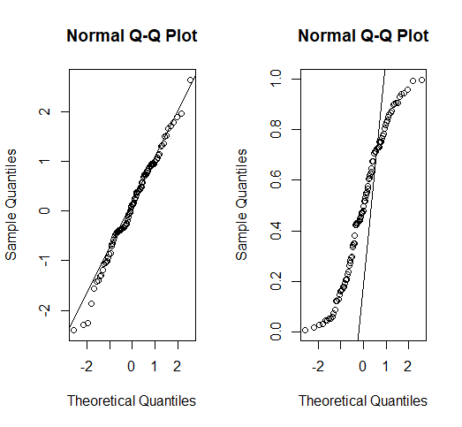
We can use the function qqnorm() which produces a quantile-quantile plot between the residuals and the theoretical values of a Normal distribution and qqline() will plot the line that would give the exact match. Complementary plots can also be used, such as histograms or density plots.
Constant variance
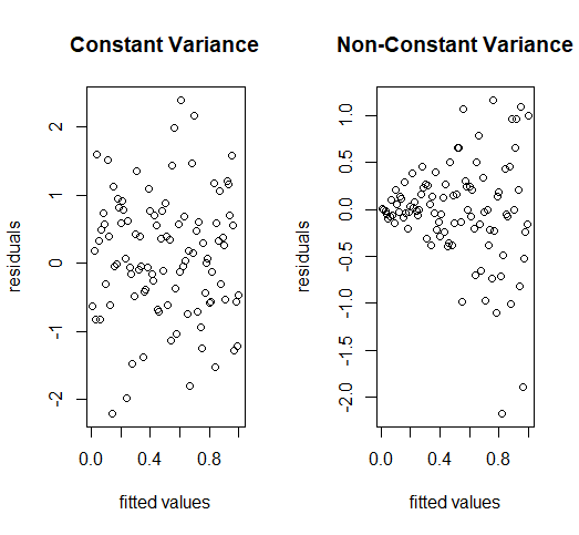
It is checked by plotting \(\hat \varepsilon_i\) versus \(\hat Y_i\). When variance is constant the residuals are scattered in a band of more or less constant width.
Linearity
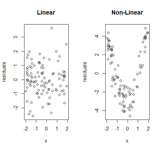
We can use similar plots as the ones used to check for constant variance:
3.2.2 Leverage and influence
Leverage is a measure of how far an observation on the predictor variable from the mean of the predictor variable. The higher the leverage value of an observation, the more potential it has to impact the fitted model
Outliers are the observations with a response \(Y_i\) is far away from the regression line. They typically do not affect the estimate of the plane, unless one of the predictors is has high leverage. But they inflate \(\hat \sigma^2\), and therefore, reduce \(R^2\)
An influential observation is an observation whose deletion has a large effect on the parameter estimates
For example, suppose that we have the follwing fitted regression model:
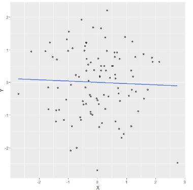 Then we will zoom out and imagine a guy trying to pull the regression line, using a rope towards him. If he moves in different locations, where will he have high potential for influence with the ablility to exert it? and where will he have high leverage but little effect on the fitted model?
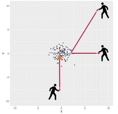
In order to measure whether an observation has an outlying value of \(\mathbf{Y}\) we use the standardized residuals, they are a modification of the residuals \(\hat \varepsilon_i\) to have unit variance. They are defined as: \[r_i=\frac{\hat \varepsilon_i}{\sqrt{\widehat{Var(\hat \varepsilon_i)}}}=\frac{\hat \varepsilon_i}{\hat\sigma\sqrt{1-h_{ii}}}.\] Another modification that make the residuals more effective in detecting outliers is to use deleted residuals. The idea is to see whether the residual changes or not when we delete the corresponding observation. If we denote \(\hat Y_{i(i)}\) the prediction when the \(i-th\) observation is deleted, the deleted residual is defined as: \[\hat \varepsilon_{(i)}=Y_i-\hat Y_{i(i)}.\] In principle, calculating \(\hat Y_{i(i)}\) could be time consuming, however it can be shown that \(\hat Y_{i(i)}=\frac{\hat \varepsilon_i}{1-h_{ii}}.\) Since the deleted residuals have no constant variance, it is preferable to use the studentized deleted residuals: \[r_i^*=\frac{\hat \varepsilon_{(i)}}{\sqrt{\widehat{Var(\hat \varepsilon_{(i)})}}}=\frac{\hat \varepsilon_{(i)}}{\hat\sigma_{(i)}\sqrt{1-h_{ii}}}.\] When the model is correct, each studentized residual follows a \(t\)-distribution with \(n-k-1\) degrees of freedom. These residuals are more appropriate to do residual plots. We will declare a point to be an outlier if the absolute value of the studentized (or standardized residual) is greater than 3.
To check whether an observation has an unusual value of the covariates, we use the hat matrix (\(\mathbf{H}\)). The diagonal elements of this matrix, \(h_{ii}\) (leverage) gives a measure of the distance of the \(i-th\) observation from the centroid of observations X. A value of \(h_{ii}\) greater that \(2(k+1)/n\) is considered high leverage, and each of these points should be investigated to see whether parameters estimates change when the \(i-th\) observation is included or excluded.
There are several measures that help us to detect influencial points, we will focus on the Cook’s Distance: \[D_i=\frac{\left ( \mathbf{\hat Y_{(i)}}- \mathbf{\hat Y} \right )^\prime\left ( \mathbf{\hat Y_{(i)}}- \mathbf{\hat Y} \right ) }{(k+1)\hat \sigma^2}=\frac{r_i^2}{(k+1)}\left ( \frac{h_{ii}}{1-h_{ii}}\right ).\] To identify potential influencial observations, one Rule of Thumb is to treat point \(i\) as influencial when: \[D_i>\frac{4}{n-k-1}. \]
Treatment of outliers/influencial observations:
The methods above only identify points that are suspicious from a statistical perspective. It does not mean that these points should automatically be eliminated!. The removal of data points can be dangerous. While this will always improve the “fit” of your regression, it may end up destroying some of the most important information in your data.
A possible approach is to perform the regression both with and without these observations, and examine their specific influence on the results. If this influence is minor, then it may not matter whether or not they are omitted. On the other hand, if their influence is substantial, then it is probably best to present the results of both analyses, and simply alert the reader to the fact that these points may be questionable.
3.2.3 Case study application
In R the functions: rstandard(), rstudent() and cooks.distance(), calculate the stardadize and studentized residuals and the Cook’s distance. Also the function influence.measures() gives further measures to detect influencial observations. If we use the function plot() on an lm object, it will return the diagnostic plots.
In the final model mod3 with only three predictors:
#Calculate influence measures
inf=influence.measures(mod3)
#Show Cook's distance and hii for the 10 first observations
inf$infmat[1:10,7:8]
##          cook.d        hat
## 1  2.833328e-02 0.05555037
## 2  1.258905e-03 0.02273942
## 3  8.408945e-05 0.03266124
## 4  5.383544e-04 0.02786396
## 5  2.174349e-02 0.20830418
## 6  6.492827e-02 0.07972759
## 7  3.304221e-03 0.04529607
## 8  6.461948e-03 0.03098681
## 9  9.585893e-04 0.03047010
## 10 9.972100e-03 0.03940056
#Check which observations could be influencial
inf$is.inf[1:10,7:8]
##    cook.d   hat
## 1   FALSE FALSE
## 2   FALSE FALSE
## 3   FALSE FALSE
## 4   FALSE FALSE
## 5   FALSE  TRUE
## 6   FALSE FALSE
## 7   FALSE FALSE
## 8   FALSE FALSE
## 9   FALSE FALSE
## 10  FALSE FALSE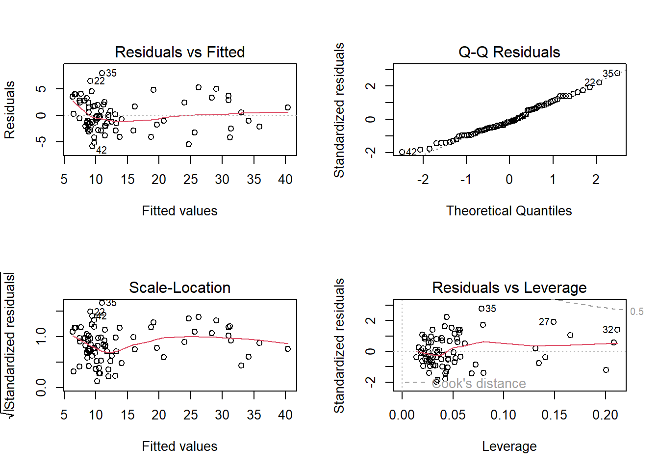
The plot on the top left corner shows if residuals have non-linear patterns. There could be a non-linear relationship between predictor variables and an outcome variable, but in this vase it might be just an artifact since most students have low values of the response variable.
The top right figure is the quantile-quantile plot and shows reasonable, although some possible observations are being pointed out as problematic.
The botton left plot is also called Spread-Location plot. This plot shows if residuals are spread equally along the ranges of predictors. This is how you can check the assumption of equal variance (homoscedasticity), again we find the same pattern.
The last plot helps us to find influential cases if any. Unlike the other plots, this time patterns are not relevant. We watch out for outlying values at the upper right corner or at the lower right corner. Those spots are the places where cases can be influential against a regression line. Look for cases outside of a dashed line, Cook’s distance. When cases are outside of the Cook’s distance (meaning they have high Cook’s distance scores), the cases are influential to the regression results. The regression results will be altered if we exclude those cases. In this case we find there is no influential case, or cases. You can barely see Cook’s distance lines (a red dashed line) because all cases are well inside of the Cook’s distance lines