Modul 7: Support Vector Machines - EKSEMPEL
library(caret)
library(ggplot2)
library(kernlab)
##
## Vedhæfter pakke: 'kernlab'
## Det følgende objekt er maskeret fra 'package:ggplot2':
##
##     alpha
library(openxlsx)
library(rsample)
library(pdp)
Klargøring af datasæt
# indlæs data
setwd(r"(C:\Users\msn.fi\OneDrive - CBS - Copenhagen Business School\Documents\AppliedMachineLearning)")

job <- read.xlsx("Jobtilfredshed.xlsx", colNames = TRUE)
job$Jobtilfredshed <- factor(job$Jobtilfredshed, levels=c("Tilfreds", "Utilfreds"))
job$Køn <- factor(job$Køn, levels = c(1, 2), labels = c("Mand","Kvinde"))
job$"Offentlig/privat" <- factor(job$"Offentlig/privat", levels = c(1, 2), labels=c("Offentlig","Privat"))
job$Region <- factor(job$Region, levels = c(1:5),
                     labels = c("Hovedstaden", "Sjælland", "Syddanmark", "Midtjylland", "Nordjylland"))
job$Motivation <- factor(job$Motivation,
                         levels = c("I mindre grad eller slet ikke", "I nogen grad", "I høj grad"),
                         ordered = TRUE)
job$Stress <- factor(job$Stress,
                     levels = c("I mindre grad eller slet ikke", "I nogen grad", "I høj grad"),
                     ordered = TRUE)
# hjælpefunktion til beregning af vip (se nedenfor)
prob_tilfreds <- function(object, newdata) {
predict(object, newdata = newdata, type = "prob")$Tilfreds
}Indledende analyse
ggplot(job,
       aes(x = Afstand.til.arbejde, fill = Jobtilfredshed, color = Jobtilfredshed)) +
  geom_histogram() +
  facet_grid(Jobtilfredshed ~ ., scales = "free_y")
## `stat_bin()` using `bins = 30`. Pick better value with `binwidth`.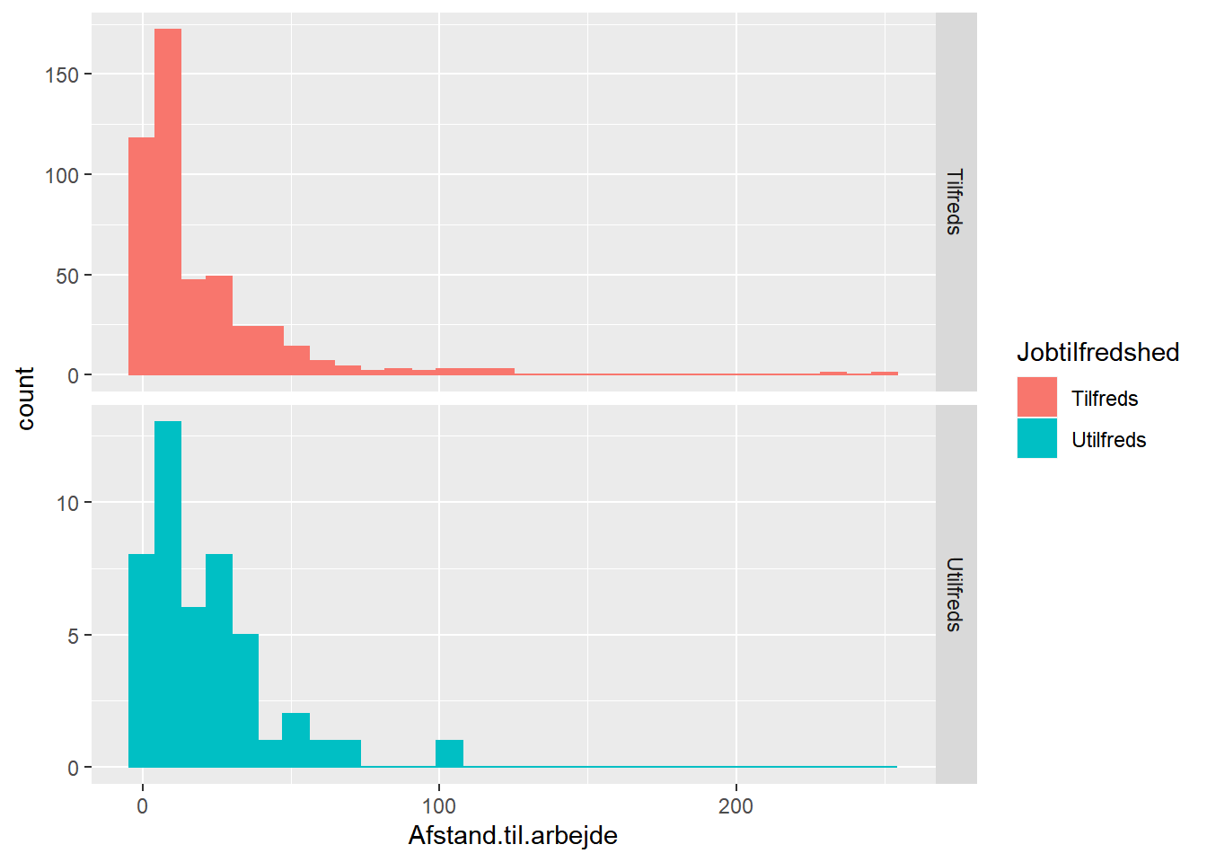
ggplot(job,
       aes(x = Arbejdstid, fill = Jobtilfredshed, color = Jobtilfredshed)) +
  geom_histogram() +
  facet_grid(Jobtilfredshed ~ ., scales = "free_y")
## `stat_bin()` using `bins = 30`. Pick better value with `binwidth`.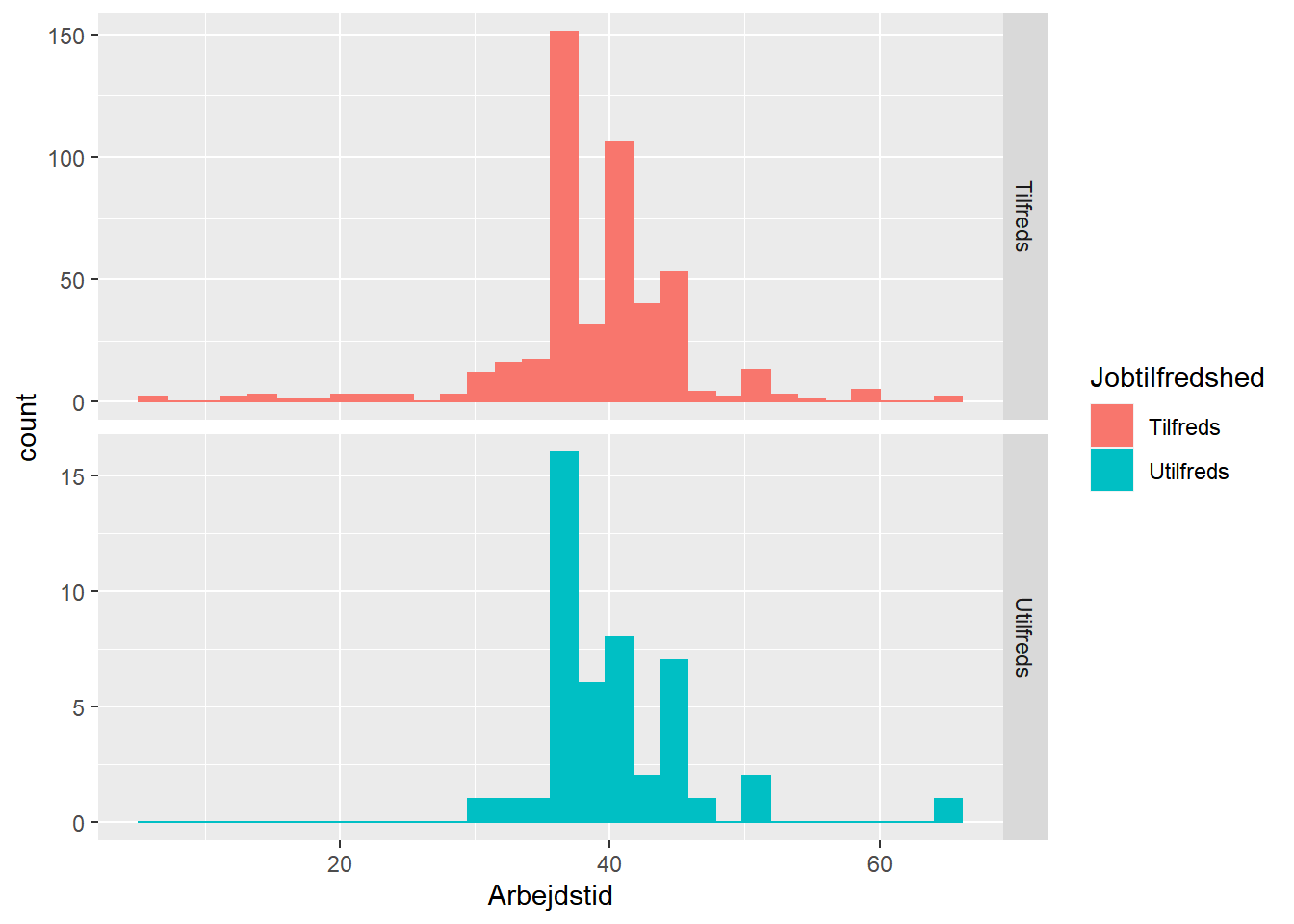
ggplot(job, aes(x = Stress, fill = Jobtilfredshed, color = Jobtilfredshed)) +
  geom_bar() +
  facet_grid(Jobtilfredshed ~ ., scales = "free_y")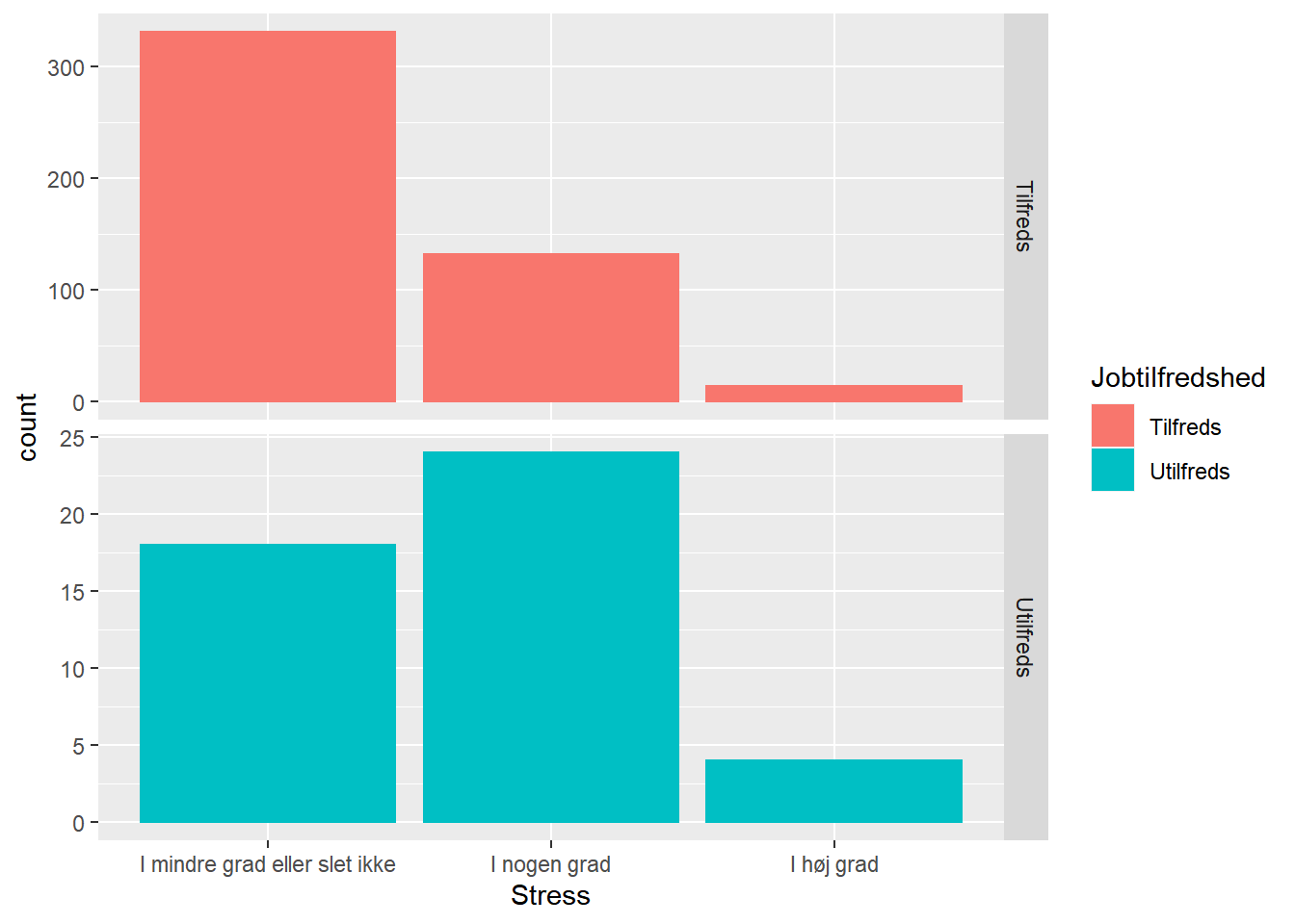
ggplot(job,
       aes(x = Motivation, fill = Jobtilfredshed, color = Jobtilfredshed)) +
  geom_bar() +
  facet_grid(Jobtilfredshed ~ ., scales = "free_y")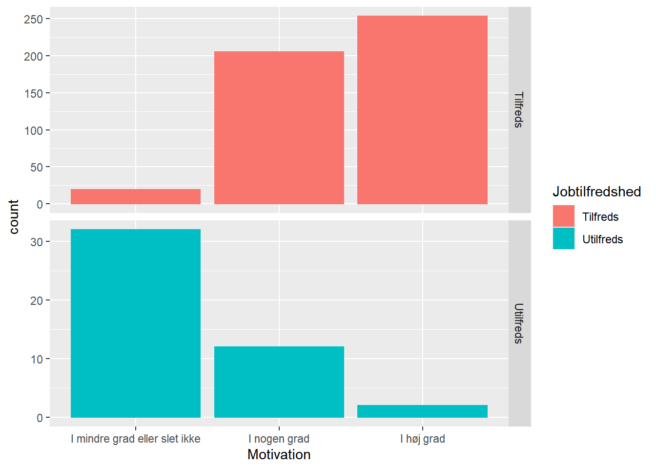
# opdeling i test- og træningsdatasæt
set.seed(4321)
split <- initial_split(job, 2/3)
train <- training(split)
test <- testing(split)
SVM med lineær kerne
# estimér SVM model
svm0 <- train(
  Jobtilfredshed ~ .,
  data = train,
  method = "svmLinear",
  preProcess = c("center", "scale"),
  metric = "ROC",
  class.weights = c("Tilfreds" = 1, "Utilfreds" = 1),
  trControl = trainControl(method = "cv", number = 10, classProbs=TRUE, summaryFunction = twoClassSummary),
  tuneLength = 10
)
Prædiktion af responsvariabel
# prædiktion af Tilfreds/Utilfreds
svm0.pred <- predict(svm0, newdata = test)
# evaluering af prædiktion v.hj.a. "confusion matrix"
svm0.confMatrix <- table(test$Jobtilfredshed, svm0.pred, dnn=c("Faktisk","Forudsagt"))
confusionMatrix(svm0.confMatrix)
## Confusion Matrix and Statistics
##
##            Forudsagt
## Faktisk     Tilfreds Utilfreds
##   Tilfreds       157         7
##   Utilfreds        2         9
##
##                Accuracy : 0.9486
##                  95% CI : (0.9046, 0.9762)
##     No Information Rate : 0.9086
##     P-Value [Acc > NIR] : 0.03653
##
##                   Kappa : 0.6398
##
##  Mcnemar's Test P-Value : 0.18242
##
##             Sensitivity : 0.9874
##             Specificity : 0.5625
##          Pos Pred Value : 0.9573
##          Neg Pred Value : 0.8182
##              Prevalence : 0.9086
##          Detection Rate : 0.8971
##    Detection Prevalence : 0.9371
##       Balanced Accuracy : 0.7750
##
##        'Positive' Class : Tilfreds
##
Prædiktion af sandsynlighed for responsvariabel
# prædiktion af sandsynlighed for Tilfreds/Utilfreds
svm0.prob <- predict(svm0, newdata=test, type="prob")

# optegn estimerede sandsynligheder opdelt på tilfredse hhv. ikke-tilfredse
hist(svm0.prob$Tilfreds[test$Jobtilfredshed=="Tilfreds"])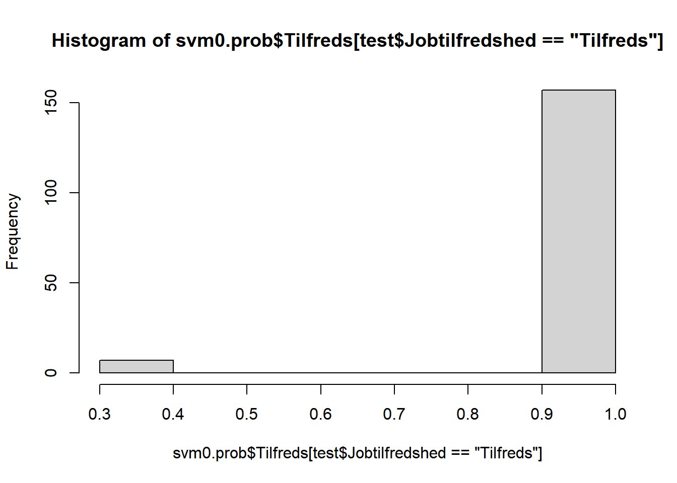
hist(svm0.prob$Tilfreds[test$Jobtilfredshed=="Utilfreds"])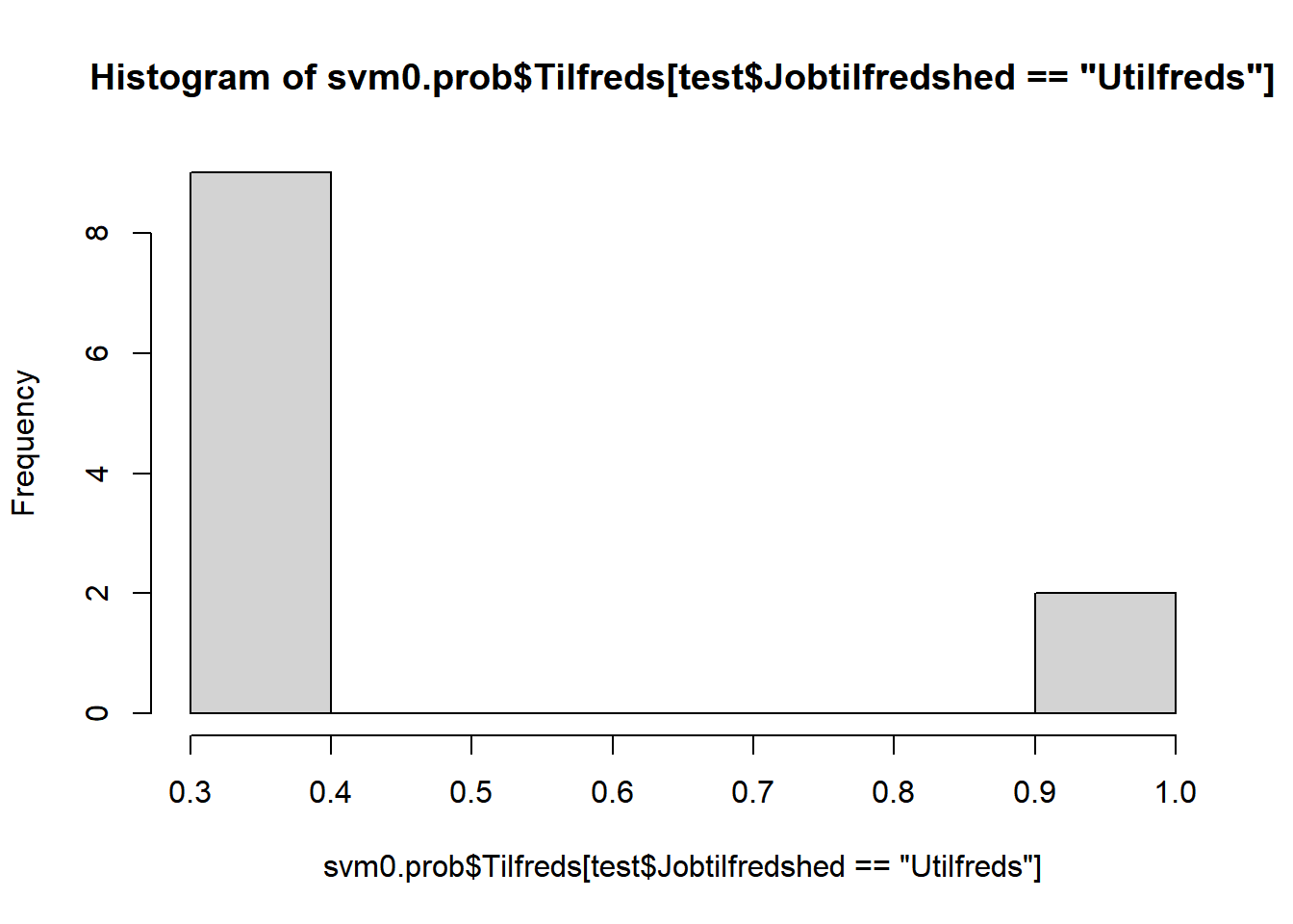
Evaluering af model fit
# tegn ROC-kurve
ROCdata <- ROCR::prediction(1 - svm0.prob$Tilfreds, test$Jobtilfredshed)
ROCkurve <- ROCR::performance(ROCdata, measure = "tpr", x.measure = "fpr")
plot(ROCkurve)
# beregning af AUC
DescTools::Cstat(x=svm0.prob$Tilfreds,
                 resp=ifelse(test$Jobtilfredshed=="Tilfreds", 1, 0))
## [1] 0.844235
# alternativ beregning af AUC
attr(ROCR::performance(ROCdata, measure = 'auc'), 'y.values')[[1]]
## [1] 0.844235
Betydning af forklarende variable
# variable importance
set.seed(2827)  # for reproducibility
vip::vip(svm0, method = "permute", nsim = 5, train = train,
    target = "Jobtilfredshed", metric = "auc", reference_class = "Tilfreds",
    pred_wrapper = prob_tilfreds)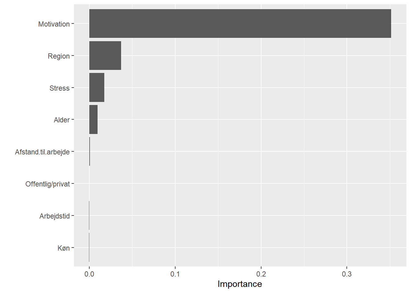
# partial dependence plots
plots <- lapply(names(train)[-1],
                function(x){partial(svm0,
                                   pred.var = x,
                                   prob = TRUE,
                                   plot = TRUE,
                                   plot.engine = 'ggplot2') + coord_flip()})
grid.arrange(grobs=plots, ncol=2)
## Warning: Use of `object[[1L]]` is discouraged. Use `.data[[1L]]` instead.
## Warning: Use of `object[["yhat"]]` is discouraged. Use `.data[["yhat"]]` instead.
## Warning: Use of `object[[1L]]` is discouraged. Use `.data[[1L]]` instead.
## Warning: Use of `object[["yhat"]]` is discouraged. Use `.data[["yhat"]]` instead.
## Warning: Use of `object[[1L]]` is discouraged. Use `.data[[1L]]` instead.
## Warning: Use of `object[["yhat"]]` is discouraged. Use `.data[["yhat"]]` instead.
## Warning: Use of `object[[1L]]` is discouraged. Use `.data[[1L]]` instead.
## Warning: Use of `object[["yhat"]]` is discouraged. Use `.data[["yhat"]]` instead.
## Warning: Use of `object[[1L]]` is discouraged. Use `.data[[1L]]` instead.
## Warning: Use of `object[["yhat"]]` is discouraged. Use `.data[["yhat"]]` instead.
## Warning: Use of `object[[1L]]` is discouraged. Use `.data[[1L]]` instead.
## Warning: Use of `object[["yhat"]]` is discouraged. Use `.data[["yhat"]]` instead.
## Warning: Use of `object[[1L]]` is discouraged. Use `.data[[1L]]` instead.
## Warning: Use of `object[["yhat"]]` is discouraged. Use `.data[["yhat"]]` instead.
## Warning: Use of `object[[1L]]` is discouraged. Use `.data[[1L]]` instead.
## Warning: Use of `object[["yhat"]]` is discouraged. Use `.data[["yhat"]]` instead.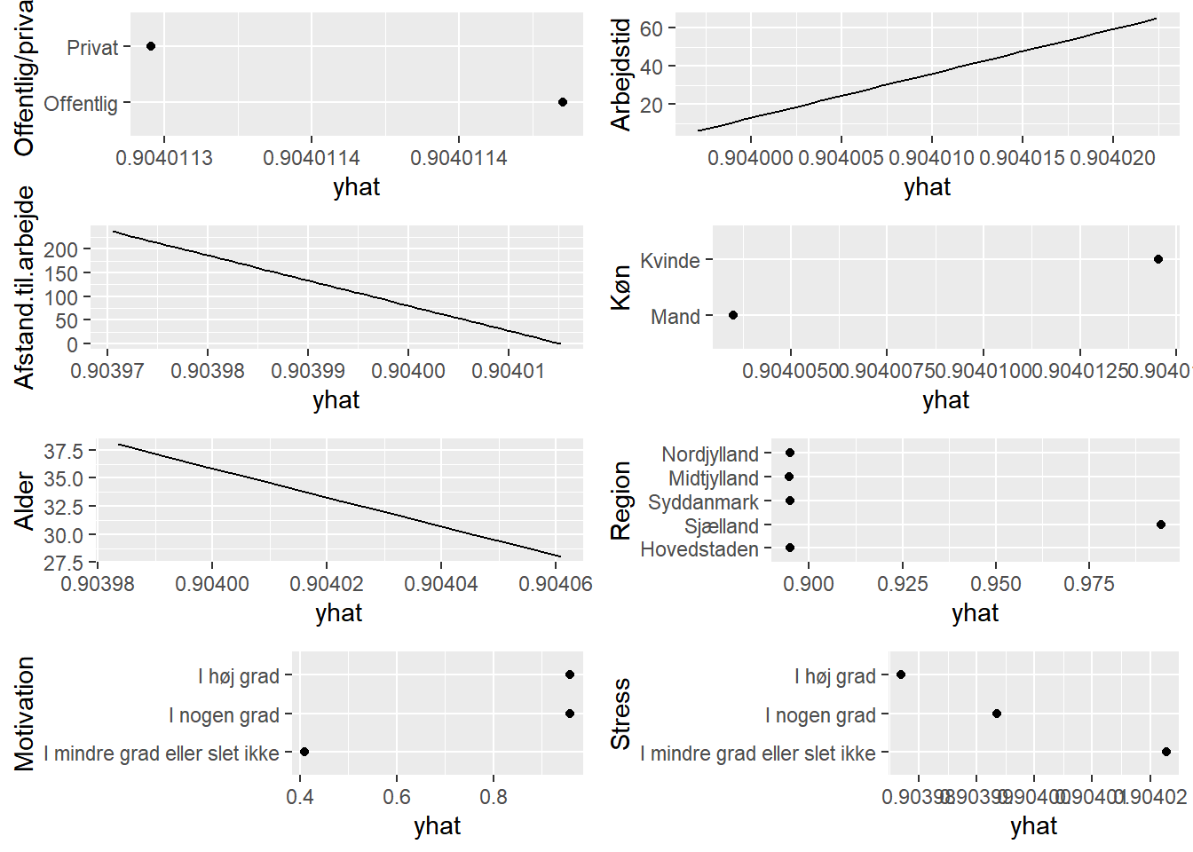
SVM med radial kerne
# estimér SVM model
svm1 <- train(
  Jobtilfredshed ~ .,
  data = train,
  method = "svmRadial",
  preProcess = c("center", "scale"),
  metric = "ROC",
  class.weights = c("Tilfreds" = 1, "Utilfreds" = 1),
  trControl = trainControl(method = "cv", number = 10, classProbs=TRUE, summaryFunction = twoClassSummary),
  tuneLength = 10
)
Prædiktion af responsvariabel
# prædiktion af Tilfreds/Utilfreds
svm1.pred <- predict(svm1, newdata = test)
# evaluering af prædiktion v.hj.a. "confusion matrix"
svm1.confMatrix <- table(test$Jobtilfredshed, svm0.pred, dnn=c("Faktisk","Forudsagt"))
confusionMatrix(svm1.confMatrix)
## Confusion Matrix and Statistics
##
##            Forudsagt
## Faktisk     Tilfreds Utilfreds
##   Tilfreds       157         7
##   Utilfreds        2         9
##
##                Accuracy : 0.9486
##                  95% CI : (0.9046, 0.9762)
##     No Information Rate : 0.9086
##     P-Value [Acc > NIR] : 0.03653
##
##                   Kappa : 0.6398
##
##  Mcnemar's Test P-Value : 0.18242
##
##             Sensitivity : 0.9874
##             Specificity : 0.5625
##          Pos Pred Value : 0.9573
##          Neg Pred Value : 0.8182
##              Prevalence : 0.9086
##          Detection Rate : 0.8971
##    Detection Prevalence : 0.9371
##       Balanced Accuracy : 0.7750
##
##        'Positive' Class : Tilfreds
##
Prædiktion af sandsynlighed for responsvariabel
# prædiktion af sandsynlighed for Tilfreds/Utilfreds
svm1.prob <- predict(svm1, newdata=test, type="prob")

# optegn estimerede sandsynligheder opdelt på tilfredse hhv. ikke-tilfredse
hist(svm1.prob$Tilfreds[test$Jobtilfredshed=="Tilfreds"])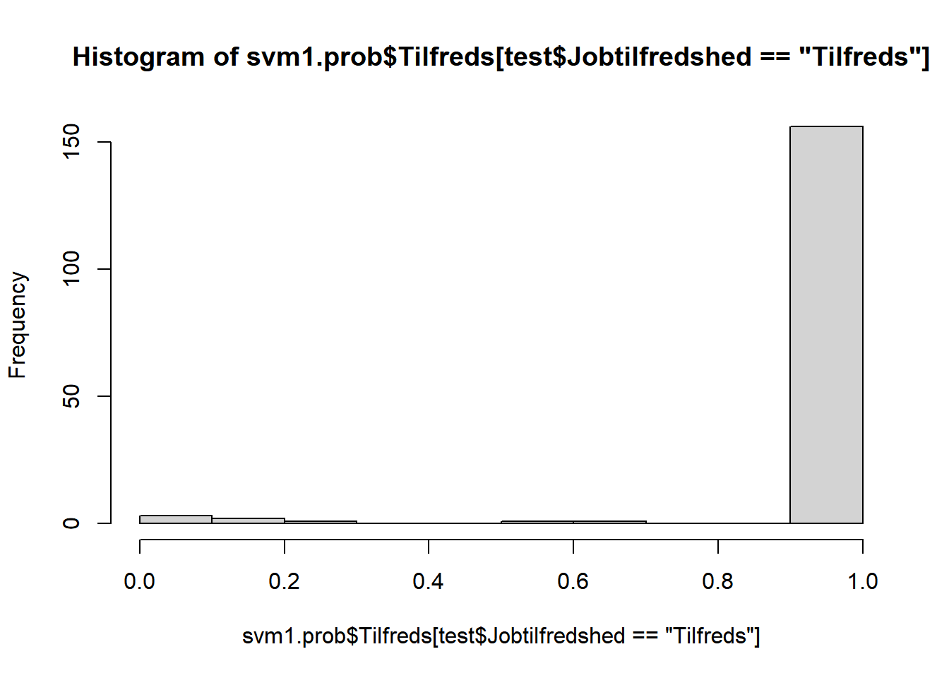
hist(svm1.prob$Tilfreds[test$Jobtilfredshed=="Utilfreds"])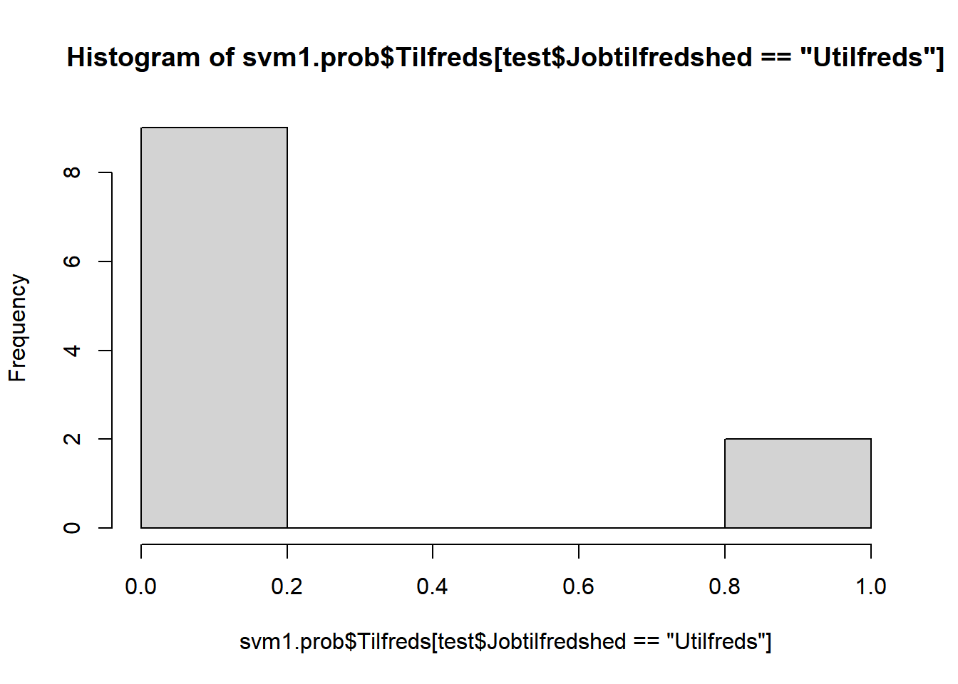
Evaluering af model fit
# tegn ROC-kurve
ROCdata <- ROCR::prediction(1 - svm1.prob$Tilfreds, test$Jobtilfredshed)
ROCkurve <- ROCR::performance(ROCdata, measure = "tpr", x.measure = "fpr")
plot(ROCkurve)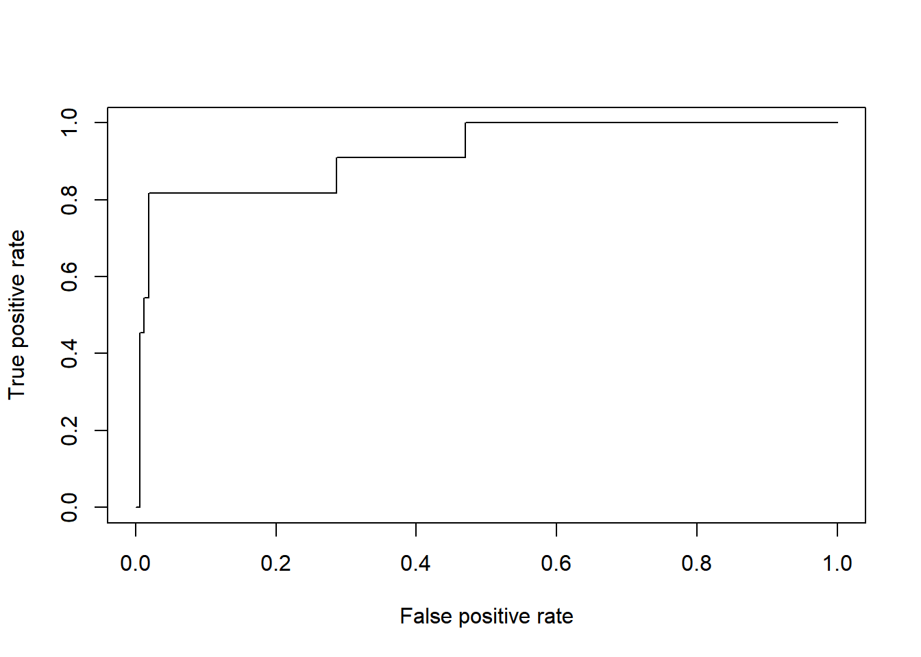
# beregning af AUC
DescTools::Cstat(x=svm1.prob$Tilfreds,
                 resp=ifelse(test$Jobtilfredshed=="Tilfreds", 1, 0))
## [1] 0.9223947
# alternativ beregning af AUC
attr(ROCR::performance(ROCdata, measure = 'auc'), 'y.values')[[1]]
## [1] 0.9223947
Betydning af forklarende variable
# variable importance
set.seed(2827)  # for reproducibility
vip::vip(svm1, method = "permute", nsim = 5, train = train,
         target = "Jobtilfredshed", metric = "auc", reference_class = "Tilfreds",
         pred_wrapper = prob_tilfreds)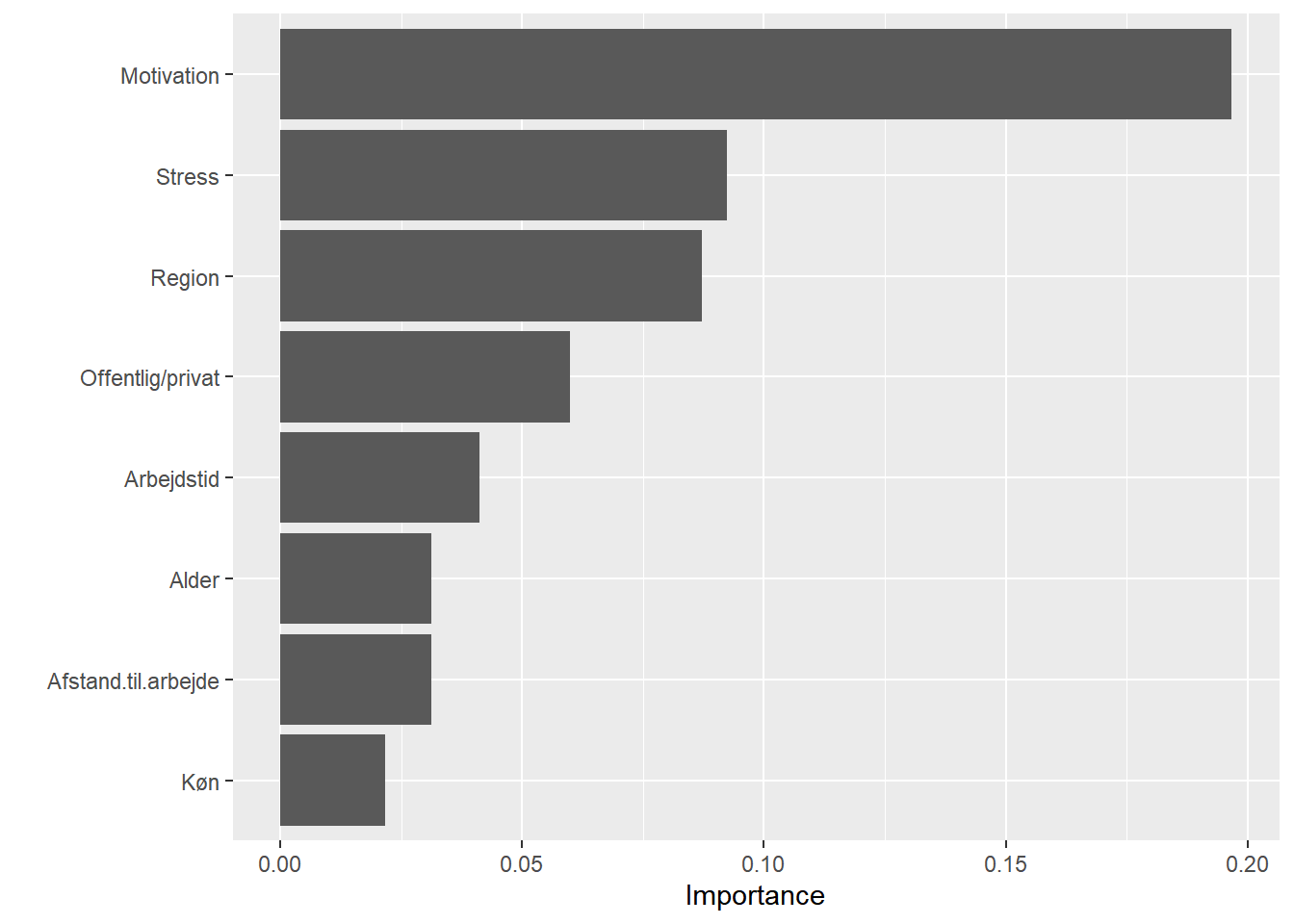
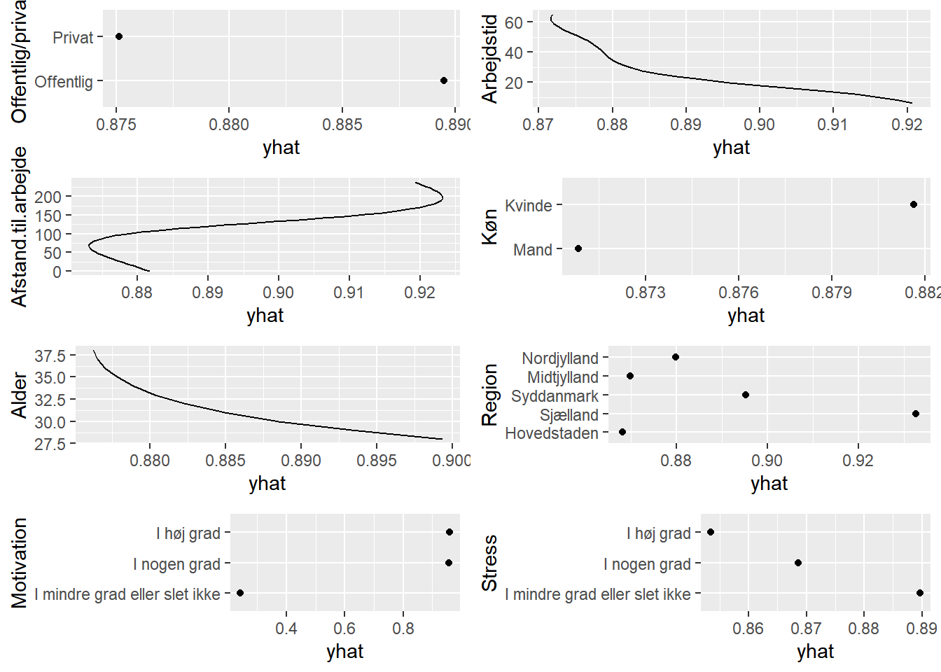
# partial dependence plots
plots <- lapply(names(train)[-1],
                function(x){partial(svm1,
                                    pred.var = x,
                                    prob = TRUE,
                                    plot = TRUE,
                                    plot.engine = 'ggplot2') + coord_flip()})
grid.arrange(grobs=plots, ncol=2)
## Warning: Use of `object[[1L]]` is discouraged. Use `.data[[1L]]` instead.
## Warning: Use of `object[["yhat"]]` is discouraged. Use `.data[["yhat"]]` instead.
## Warning: Use of `object[[1L]]` is discouraged. Use `.data[[1L]]` instead.
## Warning: Use of `object[["yhat"]]` is discouraged. Use `.data[["yhat"]]` instead.
## Warning: Use of `object[[1L]]` is discouraged. Use `.data[[1L]]` instead.
## Warning: Use of `object[["yhat"]]` is discouraged. Use `.data[["yhat"]]` instead.
## Warning: Use of `object[[1L]]` is discouraged. Use `.data[[1L]]` instead.
## Warning: Use of `object[["yhat"]]` is discouraged. Use `.data[["yhat"]]` instead.
## Warning: Use of `object[[1L]]` is discouraged. Use `.data[[1L]]` instead.
## Warning: Use of `object[["yhat"]]` is discouraged. Use `.data[["yhat"]]` instead.
## Warning: Use of `object[[1L]]` is discouraged. Use `.data[[1L]]` instead.
## Warning: Use of `object[["yhat"]]` is discouraged. Use `.data[["yhat"]]` instead.
## Warning: Use of `object[[1L]]` is discouraged. Use `.data[[1L]]` instead.
## Warning: Use of `object[["yhat"]]` is discouraged. Use `.data[["yhat"]]` instead.
## Warning: Use of `object[[1L]]` is discouraged. Use `.data[[1L]]` instead.
## Warning: Use of `object[["yhat"]]` is discouraged. Use `.data[["yhat"]]` instead.