Modul 6: Neurale netværk - EKSEMPEL
library(magrittr)
library(neuralnet)
##
## Vedhæfter pakke: 'neuralnet'
## Det følgende objekt er maskeret fra 'package:ROCR':
##
##     prediction
## Det følgende objekt er maskeret fra 'package:dplyr':
##
##     compute
library(openxlsx)
library(recipes)
library(rsample)
library(shapr)
##
## Vedhæfter pakke: 'shapr'
## Det følgende objekt er maskeret fra 'package:dplyr':
##
##     explain
Aktiveringsfunktion
# definition af sigmoid aktiveringsfunktion
sigmoid <- function(x){1/(1+exp(-x))}
# plot af logistisk/sigmoid aktiveringsfunktion
plot(x <- seq(-10,10,length=100), sigmoid(.5*x+3), type="l")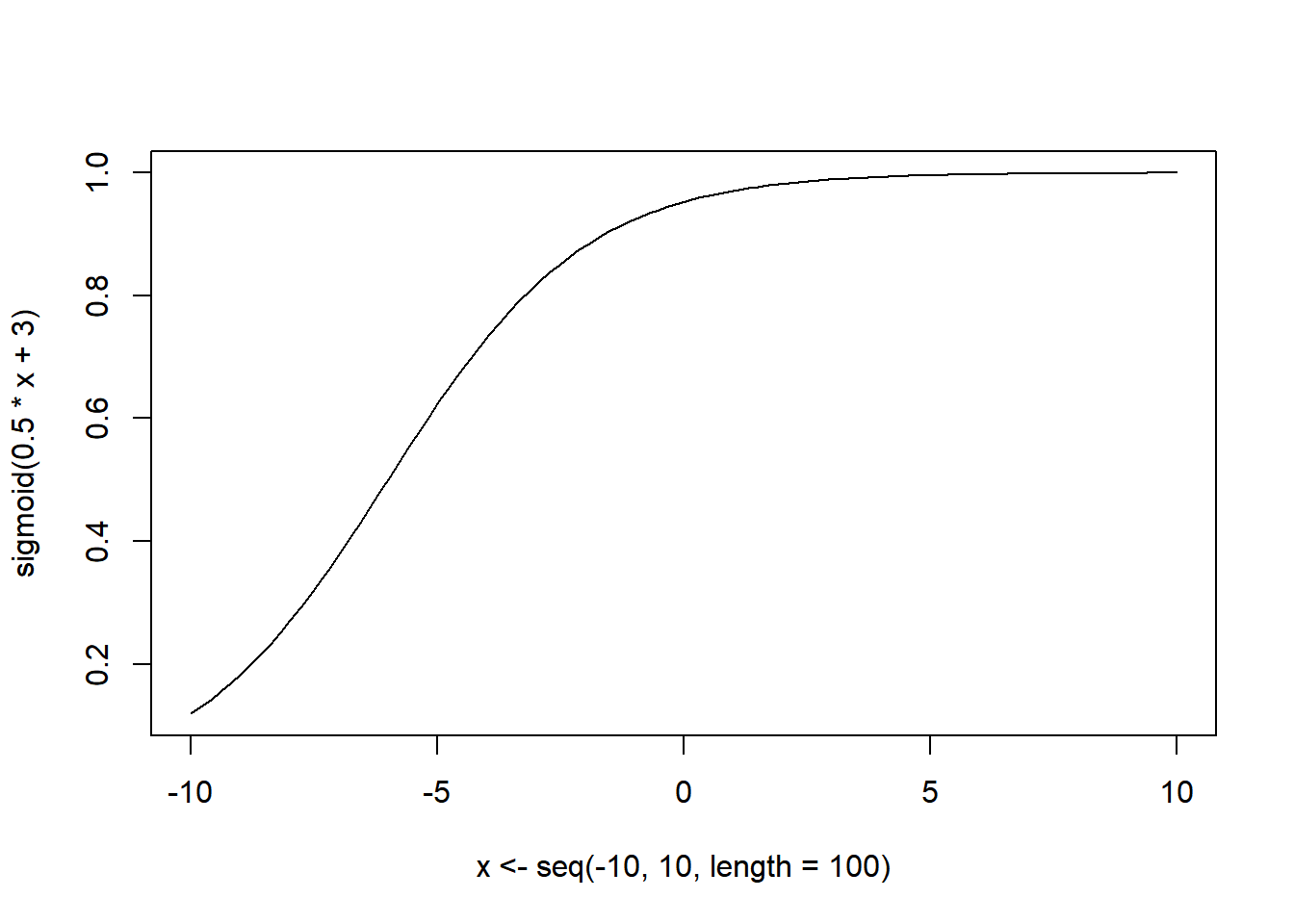
# plot af tanh aktiveringsfunktion
plot(x <- seq(-10,10,length=100), tanh(.5*x+3), type="l")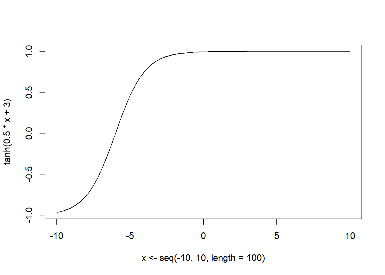
Klargøring af datasæt
# klargøring (standardisering) af datasæt [på samme måde som i modul 4]
set.seed(4321)
split <- initial_split(bolig, 2/3)
train <- training(split)
test <- testing(split)
rec <- recipe(Salgspris  ~ ., data = train) %>%
  step_date(Salgsdato, features = "decimal") %>%
  step_integer(Tidligere.solgt) %>%
  step_range(all_numeric(), min=0, max=1) %>%
  step_rm(c("Vejnavn","Husnummer","Salgsdato"))
train.std <- bake(prep(rec), train)
test.std <- bake(prep(rec), test)
View(train.std)
Indledning
Vi ser her på det simplest tænkelige neurale netværk, som har 1 input og 0 skjulte lag.
Estimation
nn <- neuralnet(Salgspris ~ Boligareal, data=train.std, hidden = 0, linear.output=TRUE)
# plot af estimeret model
dev.off(2)
## null device
##           1
plot(nn,col.entry="green",col.out="red", show.weights = T)
# modellens SSE
nn$result.matrix[c("error"),]
##    error
## 222.1333
Kontrolberegning
# input
input <- train.std$Boligareal
# bias
output.bias <- nn$weights[[1]][[1]][1]
# vægt
output.wgt <- nn$weights[[1]][[1]][2]
# prædiktion
output.result <- output.wgt*input+output.bias*1
output.result[1:5]
## [1] 0.3468929 0.3103663 0.1300162 0.2784055 0.2784055
# modellens prædiktion (for observation 1-5)
predict(nn,train.std)[1:5]
## [1] 0.3468929 0.3103663 0.1300162 0.2784055 0.2784055
Sammenligning med lineær regression
# estimation af lineær regressionsmodel
lm_fit <- lm(Salgspris ~ Boligareal, data = train.std)
# koefficienter i lineær regressionsmodel
coef(lm_fit)
## (Intercept)  Boligareal
##  0.05236006  2.25580758
# vægte i neuralt netværk
setNames(c(output.bias, output.wgt), names(coef(lm_fit)))
## (Intercept)  Boligareal
##   0.0523972   2.2555172
# vægte i neuralt netværk, når estimationspræcisionen øges
nn_accurate <- neuralnet(Salgspris ~ Boligareal, data=train.std, hidden = 0, linear.output = TRUE, threshold = 0.0000001)
setNames(nn_accurate$weights[[1]][[1]][,1], names(coef(lm_fit)))
## (Intercept)  Boligareal
##  0.05236006  2.25580759
Arkitektur
Neuralt netværk: 1 input, 1 skjult lag med 1 knude
# ~~~ Estimation ~~~
nn <- neuralnet(Salgspris ~ Boligareal, data=train.std, hidden = 1, linear.output=TRUE)
# plot af estimeret model
dev.off(2)
## null device
##           1
plot(nn,col.entry="green",col.out="red", show.weights = T)
# ~~~ Kontrolberegning (skjult lag) ~~~
# input
input <- train.std$Boligareal
# bias
hidden.bias <- nn$weights[[1]][[1]][1]
# vægt
hidden.wgt <- nn$weights[[1]][[1]][2]
# prædiktion
hidden.result <- sigmoid(hidden.wgt*input+hidden.bias*1)# ~~~ Kontrolberegning (output lag) ~~~
# bias
output.bias <- nn$weights[[1]][[2]][1]
# vægt
output.wgt <- nn$weights[[1]][[2]][2]
# prædiktion
output.result <- output.wgt*hidden.result+output.bias*1
output.result[1:5]
## [1] 0.3528739 0.2916392 0.1263348 0.2448110 0.2448110
# modellens prædiktion (for observation 1-5)
predict(nn,train.std)[1:5]
## [1] 0.3528739 0.2916392 0.1263348 0.2448110 0.2448110# ~~~ modellens fejl (= SSE/2) ~~~
nn$result.matrix[c("error"),]
## error
## 208.1507
# kontrolberegning af SSE/2
sum((train.std$Salgspris - predict(nn,train.std))^2)/2
## [1] 208.1507Neuralt netværk: 1 input, 1 skjult lag med 2 knuder
# ~~~ Estimation ~~~
nn <- neuralnet(Salgspris ~ Boligareal, data=train.std, hidden = 2, linear.output=TRUE)
# plot af estimeret model
dev.off(2)
## null device
##           1
plot(nn,col.entry="green",col.out="red", show.weights = T)
# modellens SSE
nn$result.matrix[c("error"),]
##    error
## 208.1418
# ~~~ Kontrolberegning (skjult lag) ~~~
# input
input <- train.std$Boligareal
# bias
hidden.bias <- nn$weights[[1]][[1]][1,]
# vægt
hidden.wgt <- nn$weights[[1]][[1]][2,]
# prædiktion
hidden.result <- cbind( sigmoid(hidden.wgt[1]*input+hidden.bias[1]*1),
sigmoid(hidden.wgt[2]*input+hidden.bias[2]*1) )# ~~~ Kontrolberegning (output lag) ~~~
# bias
output.bias <- nn$weights[[1]][[2]][1]
# vægte
output.wgt <- nn$weights[[1]][[2]][2:3]
# prædiktion
output.result <- output.wgt[1]*hidden.result[,1]+output.wgt[2]*hidden.result[,2]+output.bias*1
output.result[1:5]
## [1] 0.3529968 0.2921931 0.1252427 0.2454095 0.2454095
# modellens prædiktion (for observation 1-5)
predict(nn,train.std)[1:5]
## [1] 0.3529968 0.2921931 0.1252427 0.2454095 0.2454095Betydning af netværksarkitektur
nn.model1 <- neuralnet(Salgspris ~ ., data=train.std, hidden = c(5), linear.output=TRUE, threshold=0.1)
dev.off(2)
## null device
##           1
plot(nn.model1)
DescTools::RMSE(x=predict(nn.model1,test.std), ref=test.std$Salgspris)
## [1] 0.1288629

nn.model2 <- neuralnet(Salgspris ~ ., data=train.std, hidden = c(5,5), linear.output=TRUE, threshold=0.1)
dev.off(2)
## null device
##           1
plot(nn.model2)
DescTools::RMSE(x=predict(nn.model2,test.std), ref=test.std$Salgspris)
## [1] 0.1316482

nn.model3 <- neuralnet(Salgspris ~ ., data=train.std, hidden = c(5,10), linear.output=TRUE, threshold=0.1)
dev.off(2)
## null device
##           1
plot(nn.model3)
DescTools::RMSE(x=predict(nn.model3,test.std), ref=test.std$Salgspris)
## [1] 0.12941
Fortolkning af input til neuralt netværk (= forklarende variable)
# funktion til brug for beregning af Shapley-værdier
predict_model.nn <- function(x, newdata) {
  predict(x, newdata = newdata)
}
# beregning af Shapley-værdier for neuralt netværk nn.model3 (se ovenfor) for observation 1-5
nn_explainer <- shapr(train.std, nn.model3)
## get_model_specs is not available for your custom model. All feature consistency checking between model and data is disabled.
## See the 'Advanced usage' section of the vignette:
## vignette('understanding_shapr', package = 'shapr')
## for more information.
## The specified model provides feature labels that are NA. The labels of data are taken as the truth.
# NB: "as.data.frame" er nødvendig her fordi test.std ikke er en data frame
nn_shap <- explain(as.data.frame(test.std[1:5, ]),
                   nn_explainer,
                   approach = 'empirical',
                   prediction_zero = mean(train.std$Salgspris))
test.std[1:5,]
## # A tibble: 5 x 8
##   Postnummer Opførselsår Antal.værelser Grundareal Boligareal Tidligere.solgt Salgspris Salgsdato_decimal
##        <dbl>       <dbl>          <dbl>      <dbl>      <dbl>           <dbl>     <dbl>             <dbl>
## 1    0             0.861          0.211   0.00338      0.175                1     0.230             0.742
## 2    0             0.863          0.211   0.00236      0.0678               0     0.239             0.189
## 3    0.00501       0.782          0.474   0.00131      0.162                1     0.526             0.547
## 4    0.00501       0.779          0.263   0.00138      0.119                0     0.441             0.718
## 5    0.00501       0.811          0.263   0.000829     0.156                0     0.315             0.267
plot(nn_shap, index_x_test = 1:5)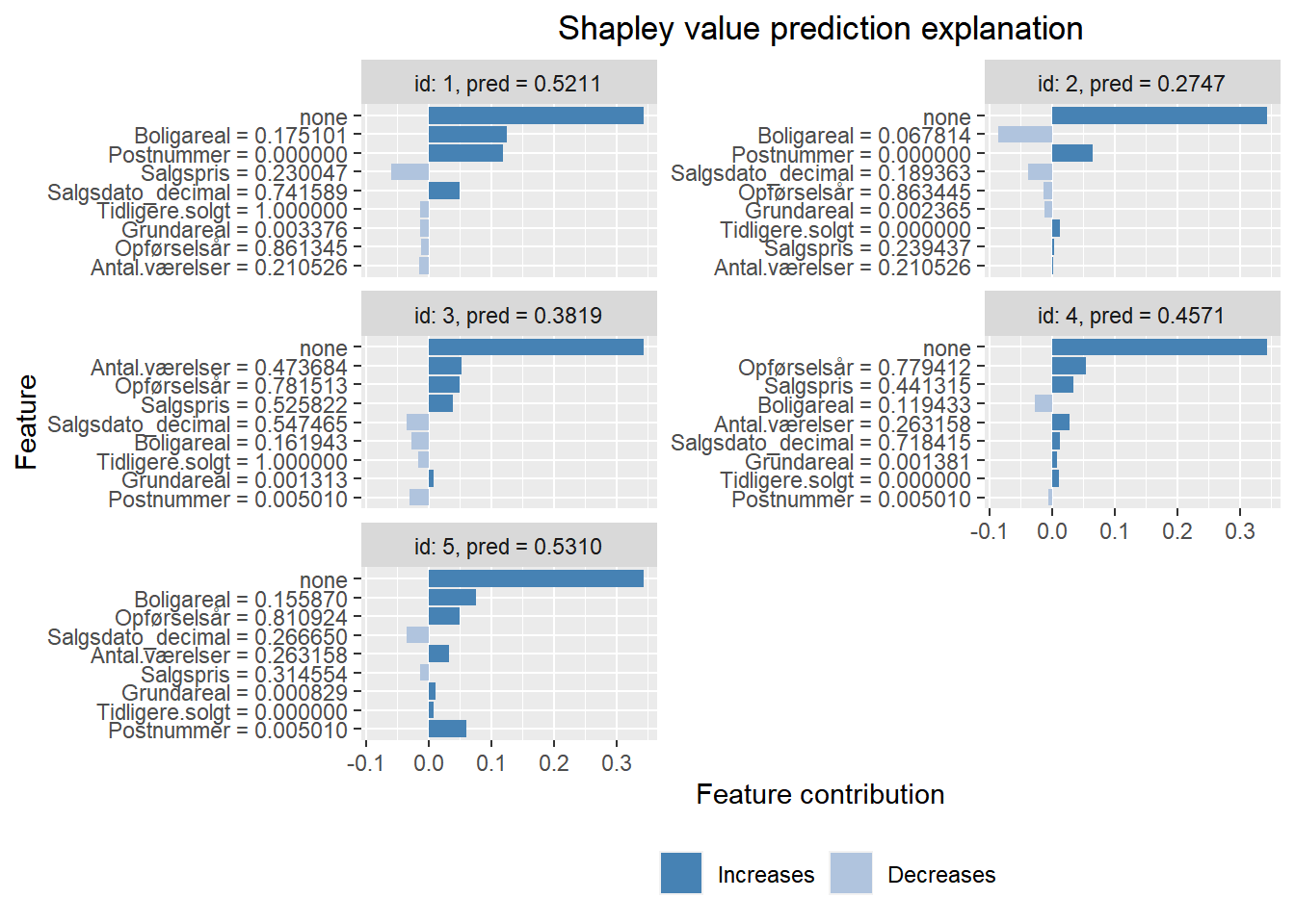
# Shapley opdeler den fittede værdi i bidrag hørende til hver enkelt forklarende variabel
nn_shap$dt
##         none   Postnummer Opførselsår Antal.værelser   Grundareal  Boligareal Tidligere.solgt    Salgspris
## 1: 0.3429702  0.118376434 -0.01204577    -0.01543997 -0.013310413  0.12553281    -0.014074836 -0.060379961
## 2: 0.3429702  0.064611623 -0.01417070     0.00183910 -0.012268266 -0.08654693     0.012874969  0.003790434
## 3: 0.3429702 -0.030308357  0.04975918     0.05217729  0.007896912 -0.02801878    -0.016759477  0.038854821
## 4: 0.3429702 -0.005485522  0.05330641     0.02762469  0.008356331 -0.02801115     0.011139276  0.034800571
## 5: 0.3429702  0.060719901  0.04967514     0.03180738  0.010494847  0.07595848     0.007333047 -0.013457145
##    Salgsdato_decimal
## 1:        0.04943960
## 2:       -0.03835143
## 3:       -0.03463261
## 4:        0.01240790
## 5:       -0.03452730
# kontrolberegning: sum af Shapley-bidrag = fittet værdi
predict(nn.model3, test.std[1:5, ])
##           [,1]
## [1,] 0.5210681
## [2,] 0.2747490
## [3,] 0.3819392
## [4,] 0.4571087
## [5,] 0.5309745
rowSums(nn_shap$dt)
## [1] 0.5210681 0.2747490 0.3819392 0.4571087 0.5309745