Chapter 4 R Lab 3 - 21/04/2021
In this lecture we will learn how to implement regression trees and one of its extensions (bagging).
The following packages are required: rpart, rpart.plot, randomForest and tidyverse.
library(rpart) #for CART
library(rpart.plot) #for plotting CART
library(randomForest) #for bagging+RF
## randomForest 4.6-14## Type rfNews() to see new features/changes/bug fixes.##
## Attaching package: 'randomForest'## The following object is masked from 'package:dplyr':
##
## combine## The following object is masked from 'package:ggplot2':
##
## marginlibrary(tidyverse) # for data management4.1 Grades data
The data we use for growing a regression tree are contained in the file grade.csv. The objective of the analysis is to predict the students’ final grade as a function of 7 regressors (e.g. age, time dedicated to study, support from school and family).
The response variable is named final_grade and is a quantitative variable.
We import the data
grade <- read.csv("/Users/marco/Google Drive Personale/Formazione/3_Unibg/2021-22/ML_tutor/RLabs/Lab4/grade.csv",sep=" ")
glimpse(grade)
## Rows: 395
## Columns: 8
## $ final_grade <dbl> 3.0, 3.0, 5.0, 7.5, 5.0, 7.5, 5.5, 3.0, 9.5, 7.5, 4.5, 6.0…
## $ age <int> 18, 17, 15, 15, 16, 16, 16, 17, 15, 15, 15, 15, 15, 15, 15…
## $ address <chr> "U", "U", "U", "U", "U", "U", "U", "U", "U", "U", "U", "U"…
## $ studytime <int> 2, 2, 2, 3, 2, 2, 2, 2, 2, 2, 2, 3, 1, 2, 3, 1, 3, 2, 1, 1…
## $ schoolsup <chr> "yes", "no", "yes", "no", "no", "no", "no", "yes", "no", "…
## $ famsup <chr> "no", "yes", "no", "yes", "yes", "yes", "no", "yes", "yes"…
## $ paid <chr> "no", "no", "yes", "yes", "yes", "yes", "no", "no", "yes",…
## $ absences <int> 6, 4, 10, 2, 4, 10, 0, 6, 0, 0, 0, 4, 2, 2, 0, 4, 6, 4, 16…Some exploratory analysis can be done to study the distribution of the regressors and of the response variable. Here below some examples follow:
grade %>%
ggplot() +
geom_histogram(aes(final_grade,after_stat(density)),bins=10)+
geom_density(aes(final_grade))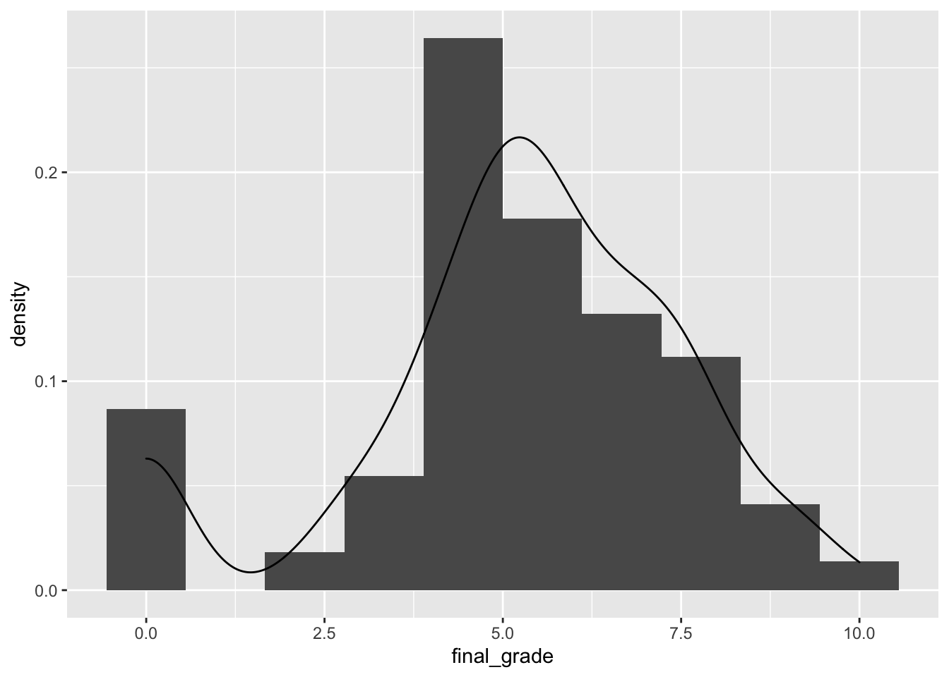 The
The final_grade distribution is characterized by two groups, the first one given by students with a grade equal to zero.
grade %>%
ggplot() +
geom_boxplot(aes(factor(studytime),final_grade,fill=factor(studytime)))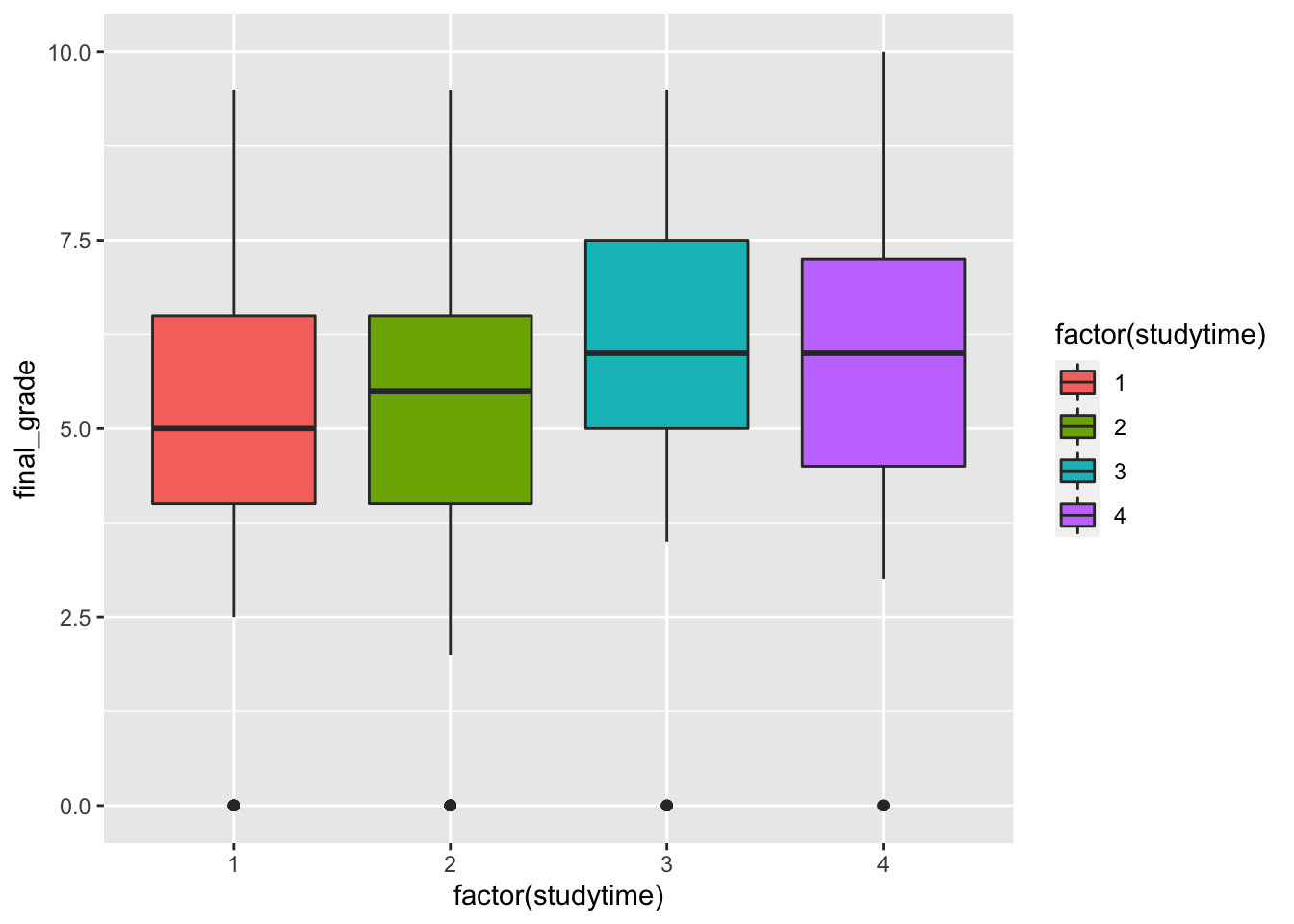 It seems that when the
 studytime variable is equal to 3 and 4 the final grades are higher. Still the group of students with a null final grade are visible as outliers.
grade %>%
ggplot() +
geom_point(aes(absences,final_grade,
col=absences>median(absences)))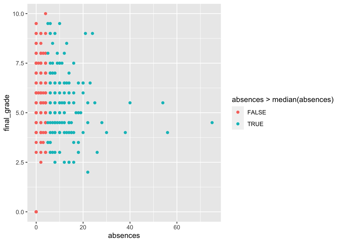 The relationship between the number of absences and the final grade is not clear. Even for students with a number of absences bigger than the median (4) the final grades have a lot of variability.
For creating the training and test sets we adopt the ones proposed in Section2.1.1.
In particular, we sample randomly for each observation (\(n\)=395) an index in the set \(\{1,2\}\), where 1 denotes the training set and 2 the test set. Obviously in this case, the sampling will be done with replacement and with different probabilities for the two numbers (0.7 and 0.3, respectively).
set.seed(1, sample.kind="Rejection")
group = sample(1:2, #1=training, 2=test
                 size = nrow(grade),
                 prob = c(0.7,0.3),
                 replace = TRUE)
head(group)
## [1] 1 1 1 2 1 2prop.table(table(group))## group
## 1 2
## 0.7139241 0.2860759We see that about 70% of the observations will be part of group 1 (training set). We are now ready to create the two separate data frames:
grade_train = grade[group == 1, ]  # subset grade to training indices only
grade_test = grade[group == 2, ]  # subset grade to test indices only
4.2 Regression tree
We use now the training data to estimate a regression tree by using the rpart function of the rpart package (see ?rpart). As usual we have to specify the formula, the dataset and the method (which will be set to anova for a regression tree). More informations about anova methodology can be find into this document (page 32).
grade_tree = rpart(formula = final_grade ~ .,
                     data = grade_train,
                     method = "anova")
Note that some options that control the rpart algorithm are specified by means of the rpart.control function (see ?rpart.control). In particular, the cp option, set by default equal to 0.01, represent a pre-pruning step because it prevents the generation of non-significant branches (any split that does not decrease the overall lack of fit by a factor of cp is not attempted). See also the meaning of the minsplit, minbucket and maxdepth options.
It is possible to plot the estimated tree as follows:
# Plot the tree model
rpart.plot(grade_tree)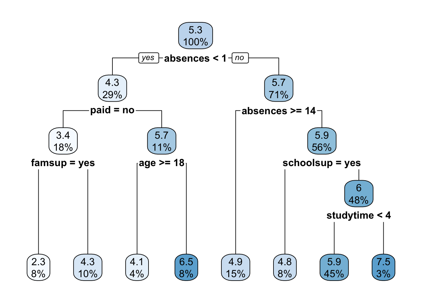 The function
 rpart.plot as different options about which information should be displayed. Here we use it with its default setting and each node provides the average grade and the percentage of observations in each node (with respect to the total number of observations). Note that basically all the numbers in the plot are rounded.
It is also possible to analyze the structure of the tree by printing it:
print(grade_tree) ## n= 282
##
## node), split, n, deviance, yval
## * denotes terminal node
##
## 1) root 282 1519.49700 5.271277
## 2) absences< 0.5 82 884.18600 4.323171
## 4) paid=no 50 565.50500 3.430000
## 8) famsup=yes 22 226.36360 2.272727 *
## 9) famsup=no 28 286.52680 4.339286 *
## 5) paid=yes 32 216.46880 5.718750
## 10) age>=17.5 10 82.90000 4.100000 *
## 11) age< 17.5 22 95.45455 6.454545 *
## 3) absences>=0.5 200 531.38000 5.660000
## 6) absences>=13.5 42 111.61900 4.904762 *
## 7) absences< 13.5 158 389.43670 5.860759
## 14) schoolsup=yes 23 50.21739 4.847826 *
## 15) schoolsup=no 135 311.60000 6.033333
## 30) studytime< 3.5 127 276.30710 5.940945 *
## 31) studytime>=3.5 8 17.00000 7.500000 *Given the grown tree we are now able to compute the predictions for the test set and to compute, as measure of performance, the mean squared error (MSE = \(\text{mean} ((y_i-\hat y_i)^2))\) with \(i\) denoting the generic observation in the test set). The predictions can be obtained by using the predict function that will return the vector of predicted grades:
grade_tree_pred = predict(object = grade_tree,
                          newdata = grade_test)
head(grade_tree_pred)
## 4 6 7 15 17 18
## 5.940945 5.940945 4.339286 2.272727 5.940945 4.847826# Compute the test MSE
mean((grade_test$final_grade - grade_tree_pred)^2)## [1] 5.2415534.3 Pruning
After the estimation of the the decision tree it is possible to remove non-significant branches (pruning) by adopting the cost-complexity approach (i.e. by penalizing for the tree size). To determine the optimal cost-complexity (CP) parameter value \(\alpha\), rpart automatically performs a 10-fold cross validation (see argument xval = 10 in the rpart.control function). The complexity table is part of the standard output of the rpart function and can be obtained as follows:
grade_tree$cptable## CP nsplit rel error xerror xstd
## 1 0.06839852 0 1.0000000 1.0066743 0.09169976
## 2 0.06726713 1 0.9316015 1.0185398 0.08663026
## 3 0.03462630 2 0.8643344 0.8923588 0.07351895
## 4 0.02508343 3 0.8297080 0.9046335 0.08045100
## 5 0.01995676 4 0.8046246 0.8920489 0.08153881
## 6 0.01817661 5 0.7846679 0.9042142 0.08283114
## 7 0.01203879 6 0.7664912 0.8833557 0.07945742
## 8 0.01000000 7 0.7544525 0.8987112 0.08200148We transform the table in a data frame in order to be able to extract more easily the information we need by means of the $ operator:
cptable = data.frame(grade_tree$cptable)Note that the number of splits is reported, rather than the number of
nodes (however remember that the number of final nodes is always given by 1 + the number of splits). The tables reports, for different values of \(\alpha\) (CP) the relative training error (rel.error) and the cross-validation error (xerror) together with its standard error (xstd). Note that the rel.error column is scaled so that the first value is 1.
The usual approach is to select the tree with the lowest cross-validation error and to find the corresponding value of CP and number of splits:
min(cptable$xerror)## [1] 0.8833557which.min(cptable$xerror) # n. of terminal nodes = position in cptable dataset## [1] 7cptable$nsplit[which.min(cptable$xerror)] #n. of split## [1] 6In this case we have that the best tree has 6 splits instead of the 7 estimated before before the post-pruning. This is not really an improvement in the simplification of the tree structure. We adopt another approach, know as “1-SE” approach which takes into account the variability of xerror resulting from cross-validation (and contained in the xstd column). We select the smallest tree whose xerror is within one standard error of the achieved minimum error (0.8833557). It means that the selected tree is the smallest tree with xerror less than the \(min(\text{xerror})+SE\), where \(min(\text{xerror})\) is the lowest estimate of the cross-validation error and \(SE\) is its corresponding standard error.
We thus define a boundary given by the minimun value of xerror plus/minus one time its xstd value:
mincpindex = which.min(cptable[,"xerror"])
LL = cptable[mincpindex,"xerror"] - cptable[mincpindex,"xstd"]
UL = cptable[mincpindex,"xerror"] + cptable[mincpindex,"xstd"]
LL
## [1] 0.8038982UL## [1] 0.9628131We know check which is the smallest tree whose xerror value is lower than the oneSElimit value:
# which n. of nodes to take into consideration?
which(cptable[,"xerror"] > LL & cptable[,"xerror"] < UL)
## [1] 3 4 5 6 7 8# which is the smallest three among them?
which(cptable[,"xerror"] > LL & cptable[,"xerror"] < UL) %>% min()## [1] 3#save the CP of our interest!
bestcp = cptable$CP[3]With this approach the best pruned has splits and the corresponding value of CP is equal to 0.0346263.
We can now prune the tree with the selected value of \(\alpha\) (CP) by using the prune function:
grade_tree_p = prune(tree = grade_tree, cp = bestcp)Let’s plot the pruned tree:
rpart.plot(x = grade_tree_p)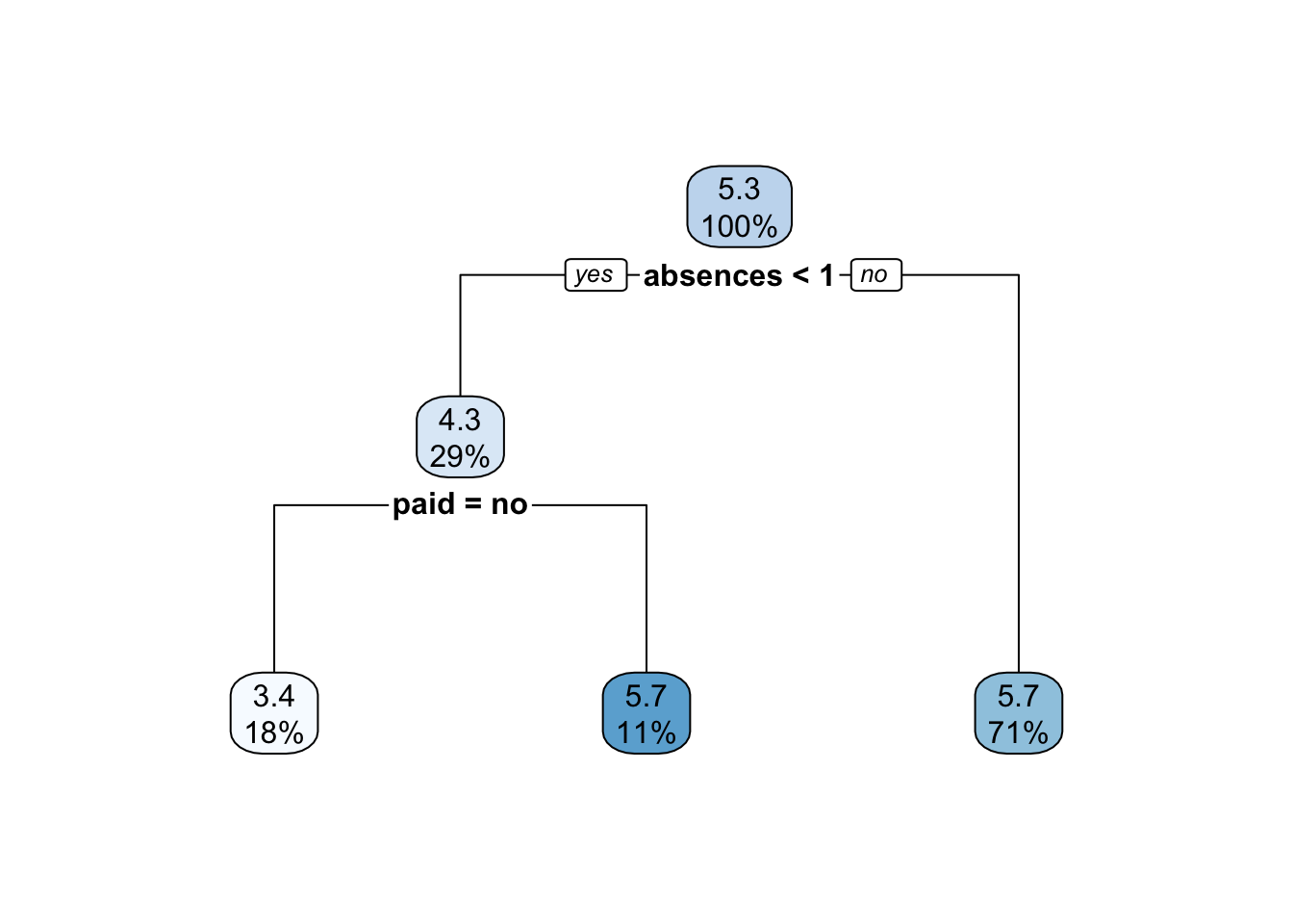
We can now compute the predictions using the pruned tree and compute the MSE:
# Generate predictions on a test set
grade_tree_pred_p = predict(object = grade_tree_p,
                          newdata = grade_test)

# Compute the Regression MSE
mean((grade_test$final_grade - grade_tree_pred_p)^2)
## [1] 4.680116# compare with unpruned MSE
mean((grade_test$final_grade - grade_tree_pred)^2)## [1] 5.241553We note that the MSE value of the pruned tree is lower than the value of the unpruned tree. Moreover, the pruned tree has a simpler structure and for this reason it should be preferred.
4.4 Bagging
Bagging corresponds to a particular case of random forest when all the regressors are used. For this reason to implement bagging we use the function randomForest in the randomForest package. As the procedure is based on boostrap resampling we need to set the seed. As usual we specify the formula and the data together with the number of regressors to be used (mtry, in this case equal to the number of columns minus the column dedicated to the response variable). **Recall to set this parameter, otherwise you are doing Random Forest! The option importance is set to T when we are interested in assessing the importance of the predictors. Finally, ntree represents the number of independent trees to grow (500 is the default value).
As bagging is based on bootstrap which is a random procedure it is convenient to set the seed before running the function:
set.seed(1, sample.kind="Rejection")
grade_bag = randomForest(formula = final_grade ~ .,
                             data = grade_train,
                             mtry = ncol(grade_train)-1, #minus the response
                             importance = T, #to estimate predictors importance
                             ntree = 500) #500 by default
grade_bag
##
## Call:
## randomForest(formula = final_grade ~ ., data = grade_train, mtry = ncol(grade_train) - 1, importance = T, ntree = 500)
## Type of random forest: regression
## Number of trees: 500
## No. of variables tried at each split: 7
##
## Mean of squared residuals: 5.021463
## % Var explained: 6.81Note that the information reported in the output (Mean of squared residuals and % Var explained) are computed using out-of-bag (OOB) observations. In particular the first figure is the last number of the mse vector provided as output of the randomForest function (the total length of the mse vector is given by the number of trees):
grade_bag$mse[500] ## [1] 5.021463As before, we compute the predictions and the test MSE:
# Generate predictions on a test set
grade_tree_bag = predict(object = grade_bag,
                          newdata = grade_test)

# Compute the test MSE
mean((grade_test$final_grade - grade_tree_bag)^2)
## [1] 4.991053Note that the MSE is slightly higher than the one obtained for the pruned tree, but still lower than the unpruned three.
Interpretability with bagging is not so straightforward as before. Still, we can assess the importance that each variable has in the reduction in RSS using the Variance Importance Plot. The highest the value, the highest the increase in RSS when the variable is excluded. So, the highest value, the more important is that variable for RSS reduction.
varImpPlot(grade_bag, type=2)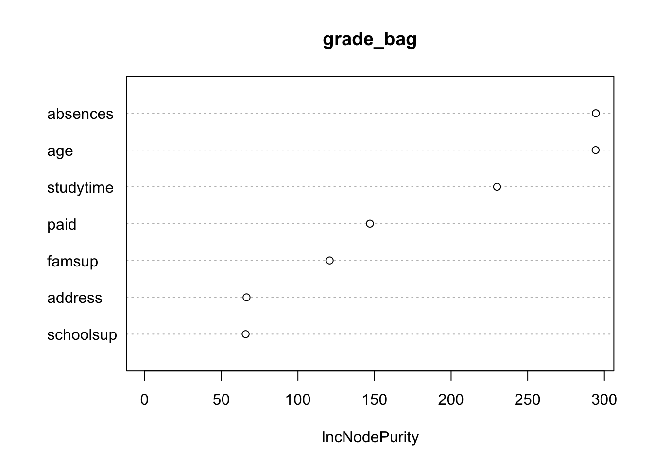
importance(grade_bag, type=2)## IncNodePurity
## age 294.32639
## address 66.46770
## studytime 229.99444
## schoolsup 65.88861
## famsup 120.73632
## paid 147.00975
## absences 294.44061In this case, Absence and Age seems to be the more important regressors.
4.5 Changing the number of bagged trees
We now analyse the effect of changing the number of trees on the OOB error. We consider in particular the sequence of the following values for the number of trees:
seq(10,1000,by=20)## [1] 10 30 50 70 90 110 130 150 170 190 210 230 250 270 290 310 330 350 370
## [20] 390 410 430 450 470 490 510 530 550 570 590 610 630 650 670 690 710 730 750
## [39] 770 790 810 830 850 870 890 910 930 950 970 990For each specific number of trees we run bagging and we extract the OOB MSE as shown before from the mse vector (it’s the last element of the vector). We run a for loop and save the OOB MSE in a vector which is initialized as an empty vector. Be careful that the process can be computational intensive!
set.seed(1, sample.kind="Rejection")
ntree_vec = seq(10,1000,by=20)
ooberrvec = c() #where we collect all the OOB mse at each iteration

for(i in 1:length(ntree_vec)){

  grade_bag = randomForest(formula = final_grade ~ .,
                             data = grade_train,
                             mtry = ncol(grade_train)-1,
                             importance = T,
                             ntree = ntree_vec[i])  #this change at each iteration
  ooberrvec[i] = grade_bag$mse[ntree_vec[i]] #extract the OOB MSE
}
We can finally plot the OOB MSE as a function of the number of trees:
plot1 <- data.frame(ntree_vec,ooberrvec) %>%
  ggplot() +
  geom_line(aes(ntree_vec,ooberrvec))+
  xlab("Number of trees")+
  ylab("OOB MSE")

plotly::ggplotly(plot1)
We can observe that starting from \(B=500\) the OOB MSE is stable (so it’s fine to run bagging with \(B=500\)).
4.6 Exercises Lab 3
4.6.1 Exercise 1
Use the Hitters dataset contained in the ISLR library. It is about Major League Baseball Data from the 1986 and 1987 seasons (322 observations of major league players on 20 variables). The main aim is to predict the annual salary of baseball players.
library(ISLR)
library(tidyverse)
?Hitters
dim(Hitters)
## [1] 322 20glimpse(Hitters)## Rows: 322
## Columns: 20
## $ AtBat <int> 293, 315, 479, 496, 321, 594, 185, 298, 323, 401, 574, 202, …
## $ Hits <int> 66, 81, 130, 141, 87, 169, 37, 73, 81, 92, 159, 53, 113, 60,…
## $ HmRun <int> 1, 7, 18, 20, 10, 4, 1, 0, 6, 17, 21, 4, 13, 0, 7, 3, 20, 2,…
## $ Runs <int> 30, 24, 66, 65, 39, 74, 23, 24, 26, 49, 107, 31, 48, 30, 29,…
## $ RBI <int> 29, 38, 72, 78, 42, 51, 8, 24, 32, 66, 75, 26, 61, 11, 27, 1…
## $ Walks <int> 14, 39, 76, 37, 30, 35, 21, 7, 8, 65, 59, 27, 47, 22, 30, 11…
## $ Years <int> 1, 14, 3, 11, 2, 11, 2, 3, 2, 13, 10, 9, 4, 6, 13, 3, 15, 5,…
## $ CAtBat <int> 293, 3449, 1624, 5628, 396, 4408, 214, 509, 341, 5206, 4631,…
## $ CHits <int> 66, 835, 457, 1575, 101, 1133, 42, 108, 86, 1332, 1300, 467,…
## $ CHmRun <int> 1, 69, 63, 225, 12, 19, 1, 0, 6, 253, 90, 15, 41, 4, 36, 3, …
## $ CRuns <int> 30, 321, 224, 828, 48, 501, 30, 41, 32, 784, 702, 192, 205, …
## $ CRBI <int> 29, 414, 266, 838, 46, 336, 9, 37, 34, 890, 504, 186, 204, 1…
## $ CWalks <int> 14, 375, 263, 354, 33, 194, 24, 12, 8, 866, 488, 161, 203, 2…
## $ League <fct> A, N, A, N, N, A, N, A, N, A, A, N, N, A, N, A, N, A, A, N, …
## $ Division <fct> E, W, W, E, E, W, E, W, W, E, E, W, E, E, E, W, W, W, W, W, …
## $ PutOuts <int> 446, 632, 880, 200, 805, 282, 76, 121, 143, 0, 238, 304, 211…
## $ Assists <int> 33, 43, 82, 11, 40, 421, 127, 283, 290, 0, 445, 45, 11, 151,…
## $ Errors <int> 20, 10, 14, 3, 4, 25, 7, 9, 19, 0, 22, 11, 7, 6, 8, 0, 10, 1…
## $ Salary <dbl> NA, 475.000, 480.000, 500.000, 91.500, 750.000, 70.000, 100.…
## $ NewLeague <fct> A, N, A, N, N, A, A, A, N, A, A, N, N, A, N, A, N, A, A, N, …Remove from the dataset the players for which
Salaryis missing. How many observation do you remove?Add to the dataset a new variable (named
logSalary) defined by the logarithmic transformation ofSalary. Then removeSalary.Plot
logSalaryas a function ofLeague. Comment the plot.Plot
logSalaryas a function ofYears. Comment the plot.Plot
logSalaryas a function ofYearsandHits(Hitson the x-axis,Yearson the y-axis and point color specified bylogSalary). Comment the plot.
Create a training set consisting of about 200 observations selected randomly, and a test set consisting of the remaining observations. Use 44 as seed.
Estimate a regression tree on the training dataset for
logSalary(use all the available predictors).Plot the tree. How many terminal nodes do you obtain?
Plot the predicted and observed logsalary data. Moreover, compute the test MSE.
By using the information contained in the
cp.tabledecide if it is convenient to prune the tree (use the 1-SE approach). If yes, evaluate the MSE for the pruned tree.Perform bagging to the Hitters training data using
logSalaryas response variable. Consider as possible values of the number of bagged trees (ntree) the regular sequence of values from 100 to 3000 with step equal to 100. Run the bagging procedure by using aforloop (one for each value ofntree) and save in a vector the values of the OOB error.Plot the the OOB MSE as a function of the number of trees:
Which is the number of trees you suggest? Compute the corresponding test MSE.
4.6.2 Exercise 2
Consider the Sales of Child Car Seats dataset (named Carseats) contained in the ISLR library`.
?Carseats

glimpse(Carseats)
## Rows: 400
## Columns: 11
## $ Sales <dbl> 9.50, 11.22, 10.06, 7.40, 4.15, 10.81, 6.63, 11.85, 6.54, …
## $ CompPrice <dbl> 138, 111, 113, 117, 141, 124, 115, 136, 132, 132, 121, 117…
## $ Income <dbl> 73, 48, 35, 100, 64, 113, 105, 81, 110, 113, 78, 94, 35, 2…
## $ Advertising <dbl> 11, 16, 10, 4, 3, 13, 0, 15, 0, 0, 9, 4, 2, 11, 11, 5, 0, …
## $ Population <dbl> 276, 260, 269, 466, 340, 501, 45, 425, 108, 131, 150, 503,…
## $ Price <dbl> 120, 83, 80, 97, 128, 72, 108, 120, 124, 124, 100, 94, 136…
## $ ShelveLoc <fct> Bad, Good, Medium, Medium, Bad, Bad, Medium, Good, Medium,…
## $ Age <dbl> 42, 65, 59, 55, 38, 78, 71, 67, 76, 76, 26, 50, 62, 53, 52…
## $ Education <dbl> 17, 10, 12, 14, 13, 16, 15, 10, 10, 17, 10, 13, 18, 18, 18…
## $ Urban <fct> Yes, Yes, Yes, Yes, Yes, No, Yes, Yes, No, No, No, Yes, Ye…
## $ US <fct> Yes, Yes, Yes, Yes, No, Yes, No, Yes, No, Yes, Yes, Yes, N…dim(Carseats)## [1] 400 11Consider
Salesas the response variable. Represent its distribution as a function ofShelveLoc.Create a dataframe for training (70% of the obs.), one for validation (15% of the obs.) and one for testing (15% of the obs.). Use 55 as seed.
Using the training data, grow a regression tree for
Sales. Plot the tree. How many terminal nodes?Have a look at the help page of
rpart.control. You will see that 20 is the default value forminsplit(the minimum number of observations that must exist in a node in order for a split to be attempted), and that 30 is the default value formaxdepth(maximum depth of any node of the final tree, with the root node counted as depth 0). In the following you have to change these default values in therpartfunction and, by using the validation data, you have to choose which is the best combination ofminsplitandmaxdepththat lead to the lowest validation MSE. Consider in particular, the following values for these 2 parameters:
# Establish a list of possible values for minsplit and maxdepth
minsplit = 1:4
maxdepth = 1:6

# Create a data frame containing all combinations
hyper_grid = expand.grid(minsplit = minsplit, maxdepth = maxdepth)

# Check out the grid of hyperparameter values
hyper_grid
## minsplit maxdepth
## 1 1 1
## 2 2 1
## 3 3 1
## 4 4 1
## 5 1 2
## 6 2 2
## 7 3 2
## 8 4 2
## 9 1 3
## 10 2 3
## 11 3 3
## 12 4 3
## 13 1 4
## 14 2 4
## 15 3 4
## 16 4 4
## 17 1 5
## 18 2 5
## 19 3 5
## 20 4 5
## 21 1 6
## 22 2 6
## 23 3 6
## 24 4 6# Number of models to run
num_models = nrow(hyper_grid)
num_models## [1] 24- Prepare an empty vector where you will save the validation MSE for each model you will run. Using a
forloop, run the 24 models that will different for the combination ofminsplitandmaxdepth(you will need an index that will cycle overhyper_grid). Compute also for each step of the loop the validation predictions and calculate the corresponding MSE that will be saved in the proper vector. At the end of the loop you will be able to identify the best model and the corresponding combination of hyper-parameters.
Given the best combination of hyper-parameters, estimate again the regression tree and compute the test error rate.
Use the results available in the
cp.tableoutput to evaluate the possibility of pruning the tree. If you decide to prune the tree, compute the new test MSE.