Chapter 9 R Lab 8 - 27/05/2022
In this lecture we will learn how to implement unsupervised methods like the principal component analysis (PCA) and clustering.
The following packages are required: MASS (included automatically in the R release), tidyverse, ggcorrplot, ggfortify, factoextra.
library(tidyverse)For this lab we will use the data contained in the file development-indicators.csv. It refers to 39 countries and 8 numerical variables including variables from The Worldwide Governance Indicators (WGI) project
about six dimensions of governance (Voice and Accountability, Political Stability and Absence of Violence/Terrorism, Government Effectiveness, Regulatory Quality, Rule of Law, Control of Corruption; see http://info.worldbank.org/governance/wgi/). We also have the GDP per capita and the total population of each country.
We start by importing the data from the csv file:
dev <- read.csv("/Users/marco/Google Drive Personale/Formazione/3_Unibg/2021-22/ML_tutor/RLabs/Lab8/development-indicators.csv")
glimpse(dev)
## Rows: 39
## Columns: 9
## $ countryname <chr> "Albania", "Austria", "Belgium", "Bulg…
## $ GDPpercapita <dbl> 5353.245, 50121.554, 46345.403, 9828.1…
## $ PopulationTotal <int> 2854191, 8879920, 11502704, 6975761, 3…
## $ WGIVoiceandAccountability <dbl> 0.151804656, 1.326598525, 1.369119644,…
## $ WGIPoliticalStabilityNoViolence <dbl> 0.1185695, 0.9801227, 0.4811862, 0.540…
## $ WGIGovernmentEffectiveness <dbl> -0.061330900, 1.490911484, 1.032227039…
## $ WGIRegulatoryQuality <dbl> 0.27437982, 1.45911550, 1.29099905, 0.…
## $ WGIRuleofLaw <dbl> -0.41117939, 1.88305128, 1.36371493, 0…
## $ WGIControlofCorruption <dbl> -0.528757572, 1.545428872, 1.551960588…Note that the first column is not numerical as it contains the names of the countries.
We first set a property of the dev dataframe which is given by the row names. Automatically they are given by the values from 1 to 39:
rownames(dev) ## [1] "1" "2" "3" "4" "5" "6" "7" "8" "9" "10" "11" "12" "13" "14" "15"
## [16] "16" "17" "18" "19" "20" "21" "22" "23" "24" "25" "26" "27" "28" "29" "30"
## [31] "31" "32" "33" "34" "35" "36" "37" "38" "39"We want instead the row names to be given by names of the countries. This will be useful later for some graphical representation:
rownames(dev) = dev$countrynameWe start the analysis with some summary statistics as the mean value and the variance for each quantitative variable:
# Compute the mean vector
dev %>%
  select_if(is.numeric) %>%
  summarise_all(mean)
## GDPpercapita PopulationTotal WGIVoiceandAccountability
## 1 32105.22 19081565 0.8020129
## WGIPoliticalStabilityNoViolence WGIGovernmentEffectiveness
## 1 0.5512366 0.8447155
## WGIRegulatoryQuality WGIRuleofLaw WGIControlofCorruption
## 1 0.960771 0.8245179 0.7254922# Compute the var vector
dev %>%
select_if(is.numeric) %>%
summarise_all(var)## GDPpercapita PopulationTotal WGIVoiceandAccountability
## 1 679811901 8.864497e+14 0.5407094
## WGIPoliticalStabilityNoViolence WGIGovernmentEffectiveness
## 1 0.3637493 0.5651742
## WGIRegulatoryQuality WGIRuleofLaw WGIControlofCorruption
## 1 0.4674545 0.7624714 0.9573218The funtion select_if is used to select only the quantitative variables and summarise_all to apply the desired function (mean or variance) to all the columns jointly. We note that the variables are caracterized by different mean and variability levels. This suggests that we will have to scale/standardize the variables.
To study the relationship between the quantitative variables (all the not the first column) we produce the plot of the correlation matrix. It is a square (8 by 8) picture whose pixels display the correlations between variables. We show only the lower part as the correlation matrix is symmetric.
library(ggcorrplot)
ggcorrplot(cor(dev[,-1]),
           hc.order = TRUE,#sort the variables
           type = "lower", #only lower part
           lab = TRUE) #display the corr values
The WGI indexes are positively and strongly correlated between themselves and also GDP. On the contrary the population size is negatively correlated with the other variables (and the values are smaller in absolute value).
9.1 Principal component analysis
We use the function prcomp to compute the principal components. In particular, with the available data we can estimate \(\min(39-1,8)=8\) PCs. We use the options center=T and scale=T in order to standardize the data and have variables with zero mean and unit variance.
pca = prcomp(dev[,-1], #only the quantitative reg.
             center = T, #zero-mean data
             scale = T) #unit variance data
The output is a list with the following components:
names(pca)## [1] "sdev" "rotation" "center" "scale" "x"The object pca$rotation contains the loadings (i.e. the \(\phi\) coefficients which define the PCs \(Z_1,Z_2,\ldots,Z_8\) as linear combination of the original variables). They are given in a 8 by 8 matrix:
pca$rotation## PC1 PC2 PC3 PC4
## GDPpercapita 0.35065863 -0.10884405 -0.65979307 -0.54248121
## PopulationTotal -0.07780194 -0.93033624 -0.06631828 0.29795108
## WGIVoiceandAccountability 0.37551195 0.02992773 0.49650096 -0.07851315
## WGIPoliticalStabilityNoViolence 0.33790638 0.28434137 -0.43261729 0.75474206
## WGIGovernmentEffectiveness 0.38985094 -0.15155311 0.02567168 0.07074205
## WGIRegulatoryQuality 0.39188875 -0.05722542 0.32191732 0.05698426
## WGIRuleofLaw 0.39825461 -0.03860397 0.14758281 0.02037978
## WGIControlofCorruption 0.38939461 -0.11466650 -0.02309969 -0.18020107
## PC5 PC6 PC7 PC8
## GDPpercapita 0.34207063 -0.02709433 0.08651057 -0.10172637
## PopulationTotal 0.15865111 0.06550130 -0.07258085 0.02279921
## WGIVoiceandAccountability 0.61814890 -0.14788749 -0.22181790 0.39017386
## WGIPoliticalStabilityNoViolence 0.15896599 0.09131232 -0.04873938 0.11041881
## WGIGovernmentEffectiveness -0.38684127 -0.74577134 0.31258960 0.12590117
## WGIRegulatoryQuality 0.05985597 0.42675083 0.66717303 -0.32473318
## WGIRuleofLaw -0.15796955 -0.05362014 -0.58666632 -0.66760776
## WGIControlofCorruption -0.52178154 0.47286419 -0.22058956 0.50764272The object pca$x contains the scores, i.e. the projection of each country on each PC. This is a 39 by 8 matrix:
pca$x## PC1 PC2 PC3 PC4
## Albania -2.81786457 0.83001739 0.05108225 -0.018111859
## Austria 2.20698529 0.15224557 0.02963347 -0.020206216
## Belgium 1.32303736 -0.01870776 0.32319894 -0.614801009
## Bulgaria -1.70556778 0.72499406 -0.01475751 0.433419354
## Bosnia and Herzegovina -3.79709805 0.71066570 -0.04188091 -0.714621571
## Belarus -4.03540331 0.69148706 -1.63463929 0.223958116
## Switzerland 3.47865606 0.04335362 -0.78991039 -0.279683041
## Czech Republic 0.39774118 0.47704781 0.21824356 0.655434401
## Germany 1.96501320 -2.40883714 0.32247456 0.260633664
## Denmark 3.01873631 0.06419015 -0.01475849 -0.304109766
## Spain 0.07977494 -0.99827534 0.43233977 0.057618727
## Estonia 1.25714266 0.41253728 0.83069018 0.006727737
## Finland 3.04903480 0.04146407 0.50805437 -0.177387799
## France 1.07966660 -1.87466237 0.41046152 -0.029540498
## United Kingdom 1.69001074 -1.86335313 0.40940542 0.111710472
## Greece -1.27759766 0.43505960 0.30629767 -0.119108855
## Croatia -1.09881576 0.83543615 -0.11148224 0.518963376
## Hungary -1.20430410 0.61702249 -0.33216718 0.579155511
## Ireland 2.31873368 0.21520412 -0.69667814 -0.668446291
## Iceland 2.81629074 0.65431469 -0.92349496 0.349248307
## Italy -0.69867269 -1.16888880 -0.03804094 0.300457221
## Lithuania 0.43699756 0.64811923 0.42977646 0.487354780
## Luxembourg 3.86050157 0.19742203 -1.63307475 -1.052842773
## Latvia 0.09629027 0.49911756 0.68497217 0.080995143
## Moldova -3.57033808 0.68928681 0.14264838 -0.638653442
## North Macedonia -2.69031446 0.71309171 0.19057057 -0.226298205
## Malta 0.34519750 0.90602080 -0.04581242 0.598224095
## Montenegro -2.29403011 0.69660531 0.08309784 -0.288168349
## Netherlands 2.80336422 -0.31506613 0.38119005 -0.182931454
## Norway 3.50279864 0.09866698 -0.32728648 -0.393764280
## Poland -0.65388391 -0.46440786 0.28125029 0.499791874
## Portugal 0.77250469 0.52038703 0.19207523 0.802437223
## Romania -1.85464178 0.43533503 -0.04141094 0.402764544
## Russian Federation -4.67157360 -3.91588928 -1.16400038 0.585045050
## Serbia -2.86654847 0.56393933 0.03073970 -0.284038079
## Slovak Republic -0.29452821 0.68211974 0.24272548 0.463753359
## Slovenia 0.57129359 0.60439086 0.21821522 0.268451833
## Sweden 3.01058493 -0.01844561 0.27916501 -0.021188677
## Ukraine -4.54917400 -1.11300876 0.81108691 -1.652242627
## PC5 PC6 PC7 PC8
## Albania 0.200474887 -0.002546889 0.248366468 0.1360118889
## Austria -0.181603079 -0.080446950 -0.249320635 -0.2336041513
## Belgium -0.001155303 0.230287837 -0.248072496 0.1178371228
## Bulgaria 0.124652221 -0.064634026 0.181718586 0.1194217216
## Bosnia and Herzegovina 0.047505355 0.214006487 -0.397973553 -0.2009921036
## Belarus -1.198305165 0.209574421 -0.005468077 0.2469325092
## Switzerland 0.044280084 -0.222770743 0.046531497 -0.0002634139
## Czech Republic 0.141771009 0.041314405 0.113632754 -0.2395791897
## Germany -0.095454353 0.281137805 -0.017567292 0.0437147654
## Denmark -0.369178252 -0.250733556 -0.134603990 0.1680749483
## Spain 0.236655891 -0.172030163 -0.078518147 -0.0356247808
## Estonia -0.471049794 0.333557102 0.146466897 0.0823879330
## Finland -0.555863358 -0.055109886 0.015239228 -0.0084845038
## France -0.060382629 -0.001684818 -0.004444178 -0.1472409098
## United Kingdom -0.177782949 0.284844489 -0.082551681 -0.0302763270
## Greece 0.529554376 -0.222929268 -0.056931031 0.2927051751
## Croatia 0.118227338 0.008129946 -0.054583063 0.0930524718
## Hungary -0.096877444 -0.067240837 0.025117567 -0.2351358037
## Ireland 0.434007322 0.163167794 0.253701778 -0.1196710146
## Iceland 0.092538336 -0.011201678 -0.260391849 0.0399224679
## Italy 0.908059152 0.216684838 0.169402818 0.2041751115
## Lithuania -0.081980599 -0.134027693 0.059654183 -0.0294204168
## Luxembourg 0.498573728 0.041236234 0.162795148 -0.0280359072
## Latvia -0.255799615 -0.296470226 0.239228566 -0.2683203000
## Moldova 0.036439257 0.079181053 -0.038049637 -0.0849354411
## North Macedonia -0.071722744 0.135793255 0.425895489 -0.1471140451
## Malta 0.500029978 -0.278440377 -0.074725422 -0.0877018477
## Montenegro -0.360036600 0.048380163 0.038213202 -0.1013204792
## Netherlands -0.291717513 0.039805509 0.142931645 0.0215738478
## Norway 0.027780376 -0.059959927 0.021406993 -0.0116389130
## Poland 0.052880188 0.312941013 0.162100234 0.1729828354
## Portugal 0.120546617 -0.312306220 -0.266819717 0.1949610022
## Romania 0.550878777 0.501754762 -0.419659237 -0.1403020154
## Russian Federation -0.142621762 -0.323862058 0.032412624 -0.1127249624
## Serbia -0.064010371 -0.160019043 -0.038239527 -0.0642576991
## Slovak Republic 0.264357349 0.018620517 0.182612043 0.0875085683
## Slovenia -0.195727167 -0.167744319 -0.155263188 0.0543467489
## Sweden -0.366194368 0.031509922 -0.003337368 0.0890345078
## Ukraine 0.108250827 -0.307768877 -0.080907633 0.1620005993We are interested in discovering which is the variability of each PC also with respect to the total variability of the original data (which is equal to 8 given that we work with scaled data):
summary(pca)## Importance of components:
## PC1 PC2 PC3 PC4 PC5 PC6 PC7
## Standard deviation 2.4691 1.0391 0.57446 0.51451 0.36396 0.20640 0.18143
## Proportion of Variance 0.7621 0.1349 0.04125 0.03309 0.01656 0.00533 0.00411
## Cumulative Proportion 0.7621 0.8970 0.93829 0.97138 0.98793 0.99326 0.99737
## PC8
## Standard deviation 0.14495
## Proportion of Variance 0.00263
## Cumulative Proportion 1.00000This table provides the standard deviation of each PC, together with the corresponding ratio with the total variability (8). The last line is the cumulative proportion of explained variance. We see that alone PC1 explains 76.21% of the total variability. If we use PC1 and PC2 we explain about 90% of the variability (and we loose about 10%). This information will be crucial for deciding how many PCs we want to keep. In this respect the screeplot is extremely useful. We provide here below two versions of the screeplot.
- The standard version of the screeplot is given by the
screeplotfunction. It displays the variance of each PC. It is evident that the first PC has the highest variability and it will contribute the most.
screeplot(pca) 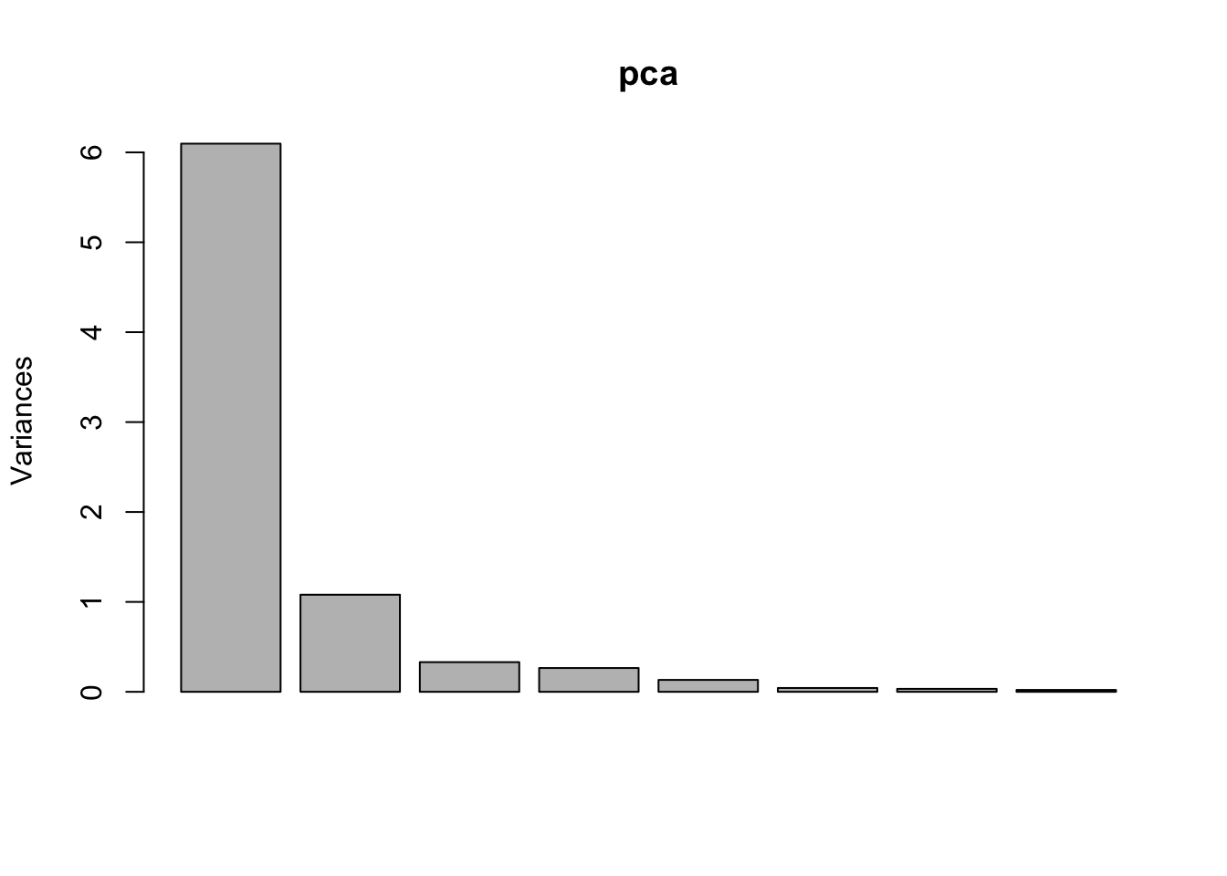
- We will display the relevant information by using
ggplot. This will require to prepare the data manually to be fed intoggplot. The dataframe we want to create has 8 rows (one for each PC) and two columns reporting the name of the PC and the cumulative proportion of explained variance (we will use thecumsumfunction for computing the cumulative sum of the PC standard deviation contained inpca$sdev):
var_explained_df = data.frame(PC = paste0("PC",1:8),
                              var_explained=(cumsum(pca$sdev^2))/sum((pca$sdev)^2))
var_explained_df
## PC var_explained
## 1 PC1 0.7620825
## 2 PC2 0.8970356
## 3 PC3 0.9382855
## 4 PC4 0.9713752
## 5 PC5 0.9879336
## 6 PC6 0.9932589
## 7 PC7 0.9973737
## 8 PC8 1.0000000var_explained_df %>%
ggplot() +
geom_point(aes(x=PC,y=var_explained),size=4) +
geom_line(aes(x=PC,y=var_explained, group="a")) +
ggtitle("Scree plot: PCA on scaled data")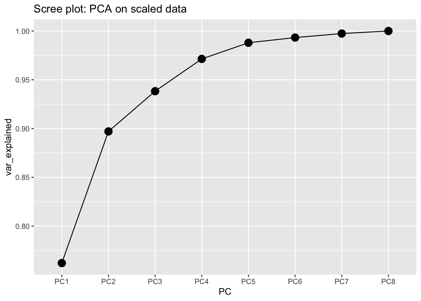
Note that we use the geometry geom_line even if on the x-axis of the plot we don’t have a quantitative variable but a factor with 8 levels. This requires to specify that all the points are of the same group and the aesthetics should be the same (group="a" where a is arbitrary).
As already seen before, the first 2 PCs explain about 90% of the variability. Including an additional PC will lead to about 94%; with 8 PCs we explain the entire variability but we are not performing any dimension reduction. We decise to keep 2 PCs and try to give an interpretation to PC1 and PC2 considering their relationship with the original variables. We start by analysis the loading
pca$rotation[,1:2]## PC1 PC2
## GDPpercapita 0.35065863 -0.10884405
## PopulationTotal -0.07780194 -0.93033624
## WGIVoiceandAccountability 0.37551195 0.02992773
## WGIPoliticalStabilityNoViolence 0.33790638 0.28434137
## WGIGovernmentEffectiveness 0.38985094 -0.15155311
## WGIRegulatoryQuality 0.39188875 -0.05722542
## WGIRuleofLaw 0.39825461 -0.03860397
## WGIControlofCorruption 0.38939461 -0.11466650The loading of PC1 are very similar for all the variables but PopulationTotal. Thus, we could conclude that PC1 is a summary of all the WGI indexes and of the wealth of a country (GDP). The loading of PC2 have a particular value which is the one referring to PopulationTotal (it is the largest in absolute value, while the others are smaller). Thus, we conclude that PC2 represents the size of a country in terms of the population. To have a confirmation of this we can plot the correlation between the scores of PC1 and the original variables using the ggcorrplot introduced before:
ggcorrplot(cor(cbind(dev[,-1],pca$x[,1])),
           hc.order = TRUE,
           type = "lower",
           lab = TRUE)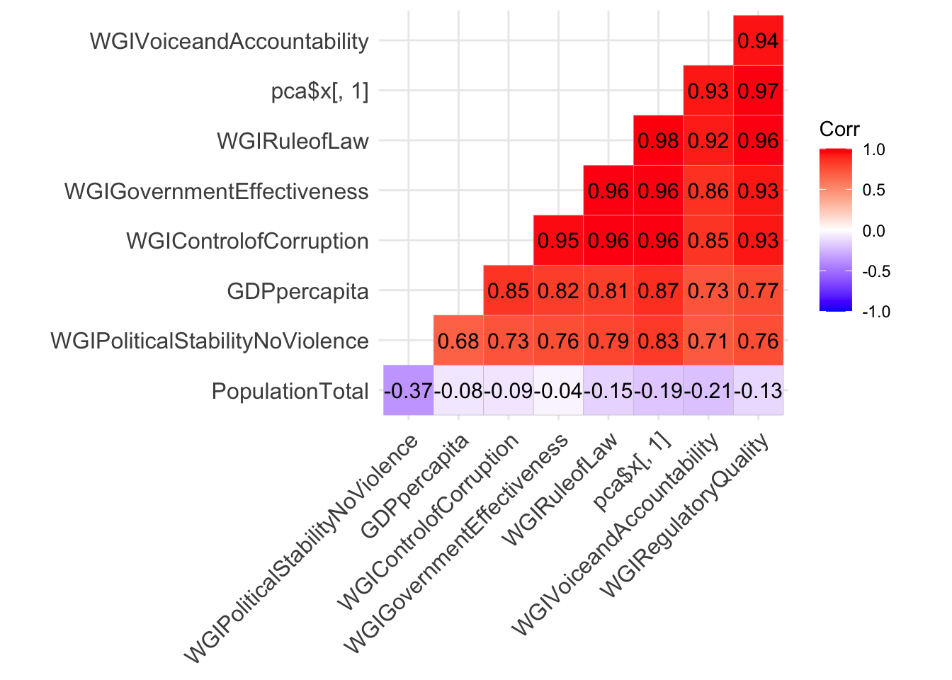
It results that PC1 is positevely and strongly correlated with the WGI variables and with GDP. The higher these variables, the higher PC1 (and viceversa). Let’s do the same for the scores of PC2:
ggcorrplot(cor(cbind(dev[,-1],pca$x[,2])),
           hc.order = TRUE,
           type = "lower",
           lab = TRUE)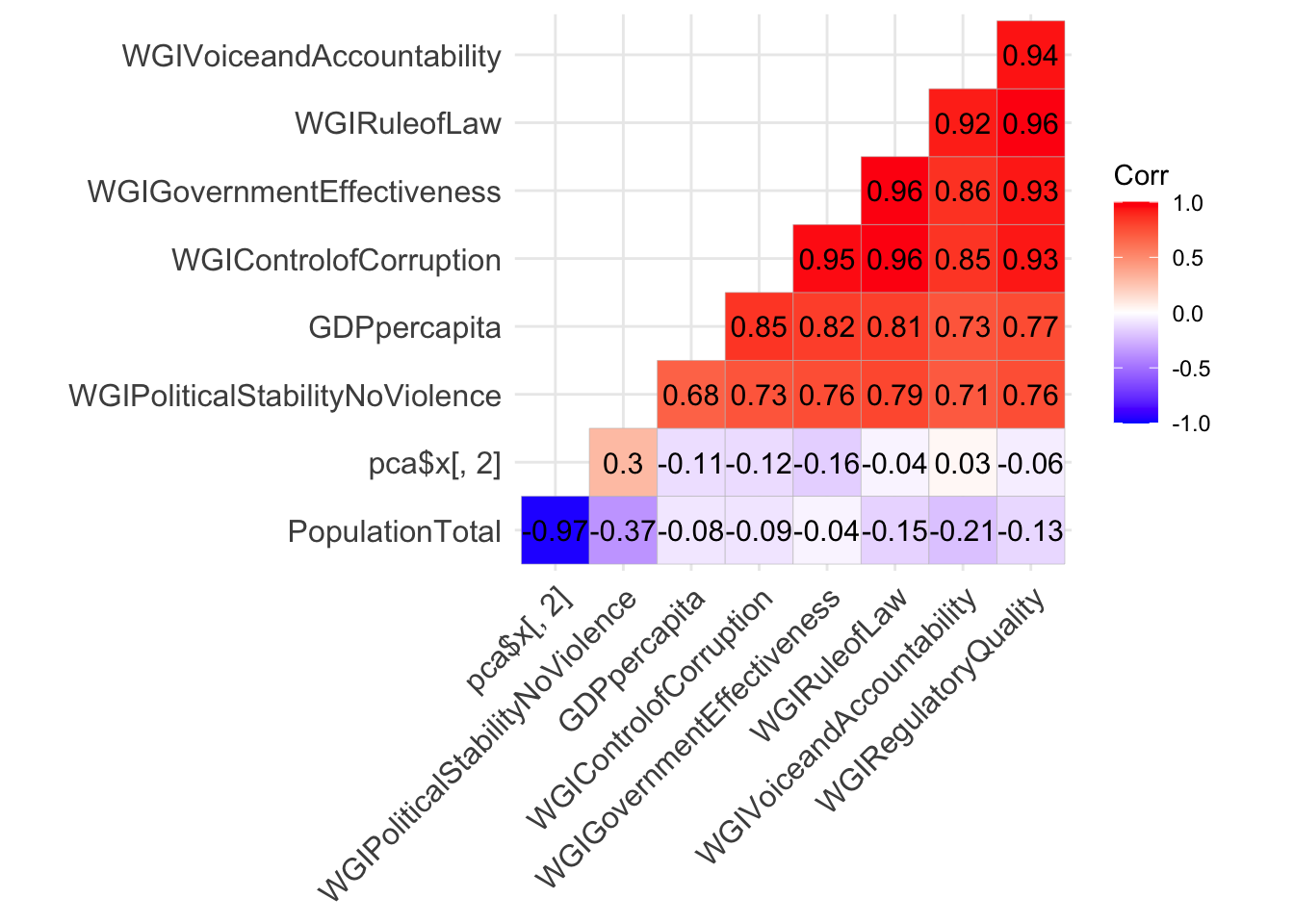
PC2 is basically uncorrelated or mildly correlated with all the variables except PopulationTotal. In fact the correlation in the latter case is equal to -0.97 (the higher the total population, the lower the PC2 score).
It’s now time to produce the biplot able to show in the same chart the loadings (referred to the original variables) and the scores (related to the countries) with respect to PC1 and PC2. We have a simple version obtained as follows:
biplot(pca,
       xlabs=dev[,1],#country names
       scale=0,#scaled data
cex=0.5) #smaller labels 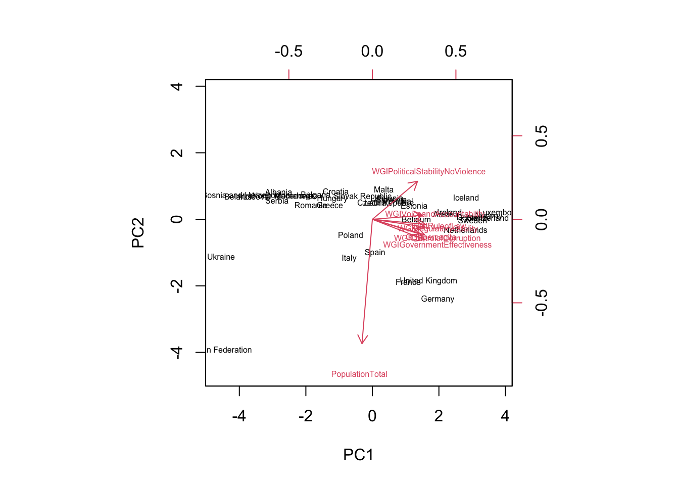
or a nicer version obtained by using the autoplot function in the ggfortify package (the interpretation will be the same):
library(ggfortify)## Warning: package 'ggfortify' was built under R version 4.0.5# this function uses the rownames of dev to get the country names
autoplot(pca,
data = dev,
scale = 0, #scaled data
label = TRUE,
loadings = TRUE,
loadings.colour = 'blue',
loadings.label = TRUE,
loadings.label.size = 3)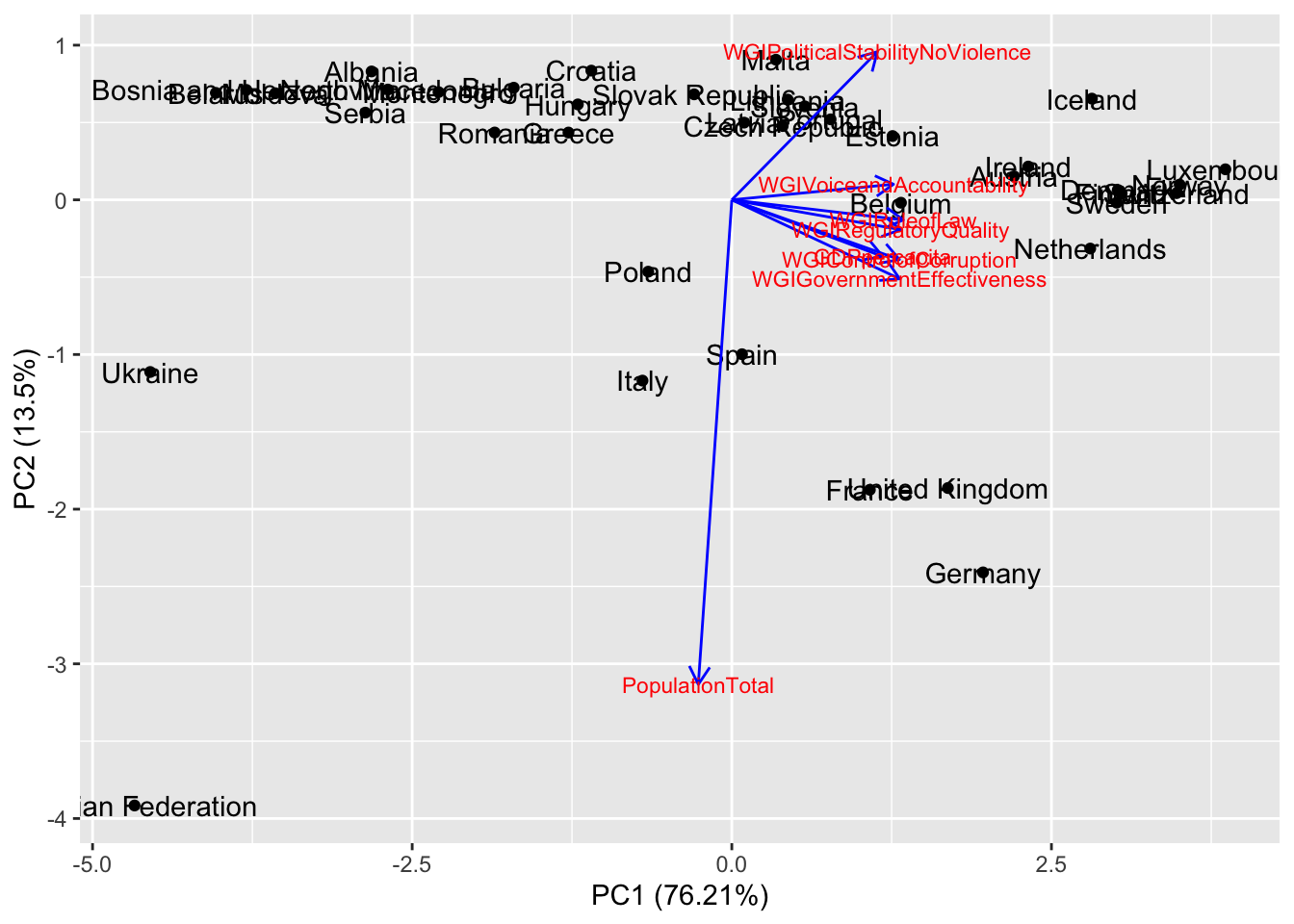
Let’s start commenting the blue arrows (loadings). The arrow pointing down (along the top-down direction of PC2) refers to PopulationTotal: we know PC2 and PopulationTotal are strongly and negatively correlated. All the other arrows are close (meaning the corresponding variables are correlated) and pointing toward right (along the left-right direction of PC1): this confirms that PC1 is explaining the WGI dimensions and the wealth of a country. Let’s move to the countries now (the scores): all the countries which lie close in the plot are similar (see for example Italy and Spain) with respect to PC1 and PC2. Russian Federation is isolated in the bottom left corner: it means that it has a large population (with respect to the average of all the countries) and a low value of wealth and governance. Ukraine has a very low value of PC1 meaning that its values of GDP and WGI indexes are below the average. We will see in the next section how to cluster the countries with respect to the available information summarized by PC1 and PC2.
9.2 Clustering
We will now implement clustering, i.e. create groups of similar countries considering the 8 original quantitative variables. We will implement both hierarchical and K-means clustering. For both the methods we need the matrix of standardized data obtained using the scale function:
scaledevnum = scale(dev[,-1])We also display, as a preliminary analysis, the distance matrix representing the similarity between the countries (using the Euclidean distance and the 8 scaled variables):
library(factoextra)## Welcome! Want to learn more? See two factoextra-related books at https://goo.gl/ve3WBafviz_dist(get_dist(scaledevnum))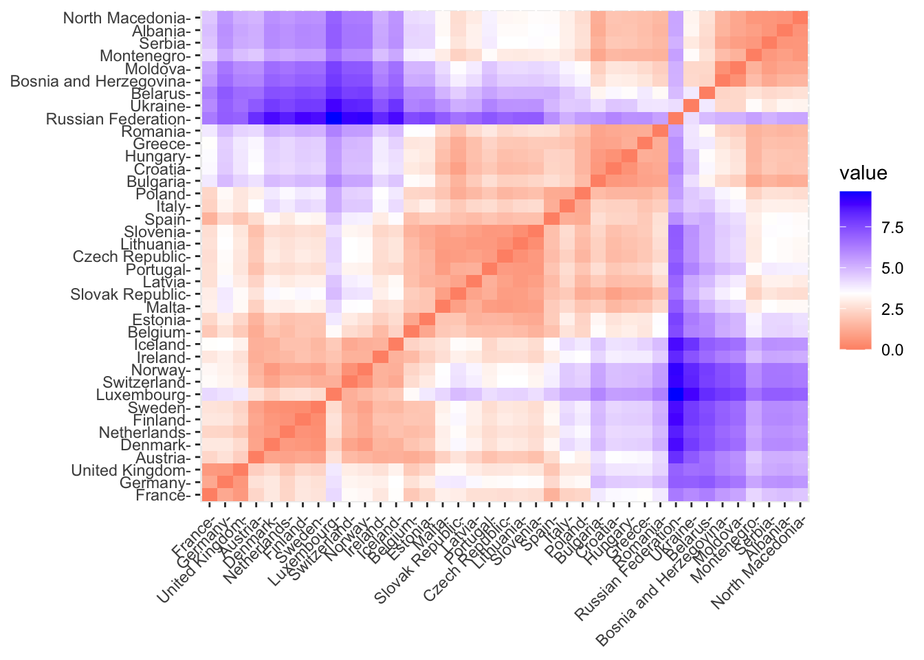 This is a 39 by 39 picture with color pixel representing the distance between two countries. The bluer the color the higher the dissimilarity. On the diagonal the distance is zero. This picture is symmetric with respect to the diagonal. We expect that similar countries will be in the same cluster.
9.2.1 Hierarchical clustering
Hierarchical clustering is implemented by the hclust function which takes in input the distance matrix obtained by dist(). It is also necessary to specify the linkage function (here below we use the complete function):
Hclusters = hclust(dist(scaledevnum),
                   method = "complete")
We immediately plot the dendogram for visualizing the clustering process (remember that we start from 39 singleton cluster and we end with 1 single big cluster):
plot(Hclusters,
     cex=0.7,#smaller text
      hang=-1) #to align at the bottom all the country names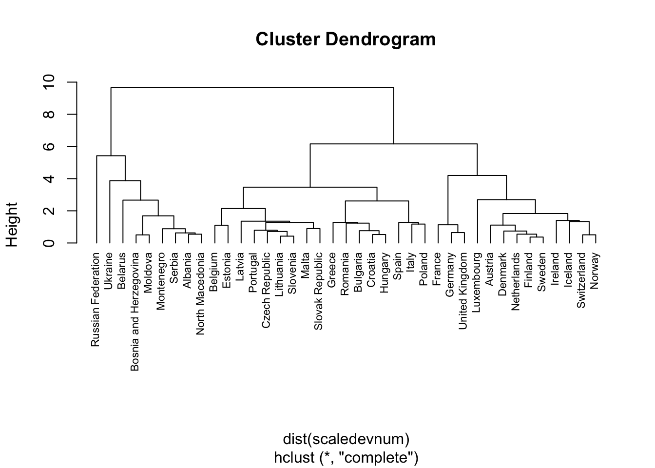
Note that the plotted country names are retrieved by the row names we set at the very beginning. Remember that the countries that join first are the most similar. We have to decide where to cut the tree (see the y-axis). We cut at the height equal to 6, but this is something that should be tuned.
HclustersCut = cutree(Hclusters, h=6)
HclustersCut
## Albania Austria Belgium
## 1 2 3
## Bulgaria Bosnia and Herzegovina Belarus
## 3 1 1
## Switzerland Czech Republic Germany
## 2 3 2
## Denmark Spain Estonia
## 2 3 3
## Finland France United Kingdom
## 2 2 2
## Greece Croatia Hungary
## 3 3 3
## Ireland Iceland Italy
## 2 2 3
## Lithuania Luxembourg Latvia
## 3 2 3
## Moldova North Macedonia Malta
## 1 1 3
## Montenegro Netherlands Norway
## 1 2 2
## Poland Portugal Romania
## 3 3 3
## Russian Federation Serbia Slovak Republic
## 1 1 3
## Slovenia Sweden Ukraine
## 3 2 1HclustersCut contains the specification of the corresponding cluster for each country. We can thus count how many countries we have in each cluster and arrange the countries by cluster:
table(HclustersCut)## HclustersCut
## 1 2 3
## 9 13 17data.frame(HclustersCut) %>% arrange(HclustersCut)## HclustersCut
## Albania 1
## Bosnia and Herzegovina 1
## Belarus 1
## Moldova 1
## North Macedonia 1
## Montenegro 1
## Russian Federation 1
## Serbia 1
## Ukraine 1
## Austria 2
## Switzerland 2
## Germany 2
## Denmark 2
## Finland 2
## France 2
## United Kingdom 2
## Ireland 2
## Iceland 2
## Luxembourg 2
## Netherlands 2
## Norway 2
## Sweden 2
## Belgium 3
## Bulgaria 3
## Czech Republic 3
## Spain 3
## Estonia 3
## Greece 3
## Croatia 3
## Hungary 3
## Italy 3
## Lithuania 3
## Latvia 3
## Malta 3
## Poland 3
## Portugal 3
## Romania 3
## Slovak Republic 3
## Slovenia 3The first cluster, containing 9 countries, is the one displayed on the left in the dendrogram (with Russian Federation and North Macedonia). The second cluster is composed by 13 countries including Austria and Norway (it’s on the right in the dendrogram). The last one, with 17 countries, include Italy and Spain.
9.2.2 K-means clustering
With K-means clustering we have to specify how many clusters we want to create, we will try with 3 (see the centers option of the kmeans function). As the final solution is sensitive to the starting point we run the algorithm nstart times (automatically the bset solution with the lowest total within sum of squares will be returned):
set.seed(44)
cl3 = kmeans(scaledevnum,
            centers = 3, #n. of clusters
            iter.max = 1000,
            nstart = 25) #run the alg. 25 times
We check the final clustering as follows
cl3## K-means clustering with 3 clusters of sizes 9, 15, 15
##
## Cluster means:
## GDPpercapita PopulationTotal WGIVoiceandAccountability
## 1 -0.9746276 0.16773189 -1.47343645
## 2 -0.4348758 -0.12587149 0.03634483
## 3 1.0196523 0.02523236 0.84771704
## WGIPoliticalStabilityNoViolence WGIGovernmentEffectiveness
## 1 -1.3878111 -1.3062546
## 2 0.2149136 -0.2161675
## 3 0.6177731 0.9999202
## WGIRegulatoryQuality WGIRuleofLaw WGIControlofCorruption
## 1 -1.4305953 -1.3897438 -1.2237505
## 2 -0.1109633 -0.1795747 -0.3856619
## 3 0.9693205 1.0134210 1.1199122
##
## Clustering vector:
## Albania Austria Belgium
## 1 3 3
## Bulgaria Bosnia and Herzegovina Belarus
## 2 1 1
## Switzerland Czech Republic Germany
## 3 2 3
## Denmark Spain Estonia
## 3 2 3
## Finland France United Kingdom
## 3 3 3
## Greece Croatia Hungary
## 2 2 2
## Ireland Iceland Italy
## 3 3 2
## Lithuania Luxembourg Latvia
## 2 3 2
## Moldova North Macedonia Malta
## 1 1 2
## Montenegro Netherlands Norway
## 1 3 3
## Poland Portugal Romania
## 2 2 2
## Russian Federation Serbia Slovak Republic
## 1 1 2
## Slovenia Sweden Ukraine
## 2 3 1
##
## Within cluster sum of squares by cluster:
## [1] 35.96384 21.34451 33.57328
## (between_SS / total_SS = 70.1 %)
##
## Available components:
##
## [1] "cluster" "centers" "totss" "withinss" "tot.withinss"
## [6] "betweenss" "size" "iter" "ifault"data.frame(cl3$cluster) %>% arrange(cl3.cluster)## cl3.cluster
## Albania 1
## Bosnia and Herzegovina 1
## Belarus 1
## Moldova 1
## North Macedonia 1
## Montenegro 1
## Russian Federation 1
## Serbia 1
## Ukraine 1
## Bulgaria 2
## Czech Republic 2
## Spain 2
## Greece 2
## Croatia 2
## Hungary 2
## Italy 2
## Lithuania 2
## Latvia 2
## Malta 2
## Poland 2
## Portugal 2
## Romania 2
## Slovak Republic 2
## Slovenia 2
## Austria 3
## Belgium 3
## Switzerland 3
## Germany 3
## Denmark 3
## Estonia 3
## Finland 3
## France 3
## United Kingdom 3
## Ireland 3
## Iceland 3
## Luxembourg 3
## Netherlands 3
## Norway 3
## Sweden 3table(cl3$cluster)##
## 1 2 3
## 9 15 15We use the following code for plotting the clustering. As we are considering 8 variables it is not possible to create a plot in 8 dimensions. The function autoplot automatically performs a dimension reduction with… PCA! The first two PC2 are used for the graphical representation. They are the same PCs that we have commented about in the previous section.
autoplot(cl3,
         data = scaledevnum,
         scale = 0,#scaled data
         label = TRUE,
         frame = TRUE,
         frame.type = "norm")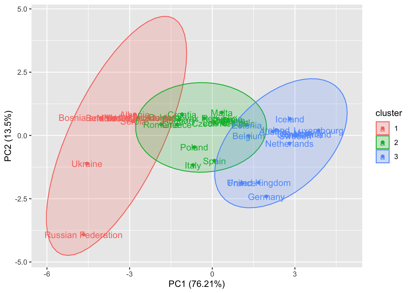
What we obtain is very similar to the output of the hierarchical clustering with the dendrogram cut at 6.
We know that K-means algorithm minimizes the total within cluster variability (and at the same time to maximize the between cluster variability). This information is given in the last part of the output of kmeans:
cl3## K-means clustering with 3 clusters of sizes 9, 15, 15
##
## Cluster means:
## GDPpercapita PopulationTotal WGIVoiceandAccountability
## 1 -0.9746276 0.16773189 -1.47343645
## 2 -0.4348758 -0.12587149 0.03634483
## 3 1.0196523 0.02523236 0.84771704
## WGIPoliticalStabilityNoViolence WGIGovernmentEffectiveness
## 1 -1.3878111 -1.3062546
## 2 0.2149136 -0.2161675
## 3 0.6177731 0.9999202
## WGIRegulatoryQuality WGIRuleofLaw WGIControlofCorruption
## 1 -1.4305953 -1.3897438 -1.2237505
## 2 -0.1109633 -0.1795747 -0.3856619
## 3 0.9693205 1.0134210 1.1199122
##
## Clustering vector:
## Albania Austria Belgium
## 1 3 3
## Bulgaria Bosnia and Herzegovina Belarus
## 2 1 1
## Switzerland Czech Republic Germany
## 3 2 3
## Denmark Spain Estonia
## 3 2 3
## Finland France United Kingdom
## 3 3 3
## Greece Croatia Hungary
## 2 2 2
## Ireland Iceland Italy
## 3 3 2
## Lithuania Luxembourg Latvia
## 2 3 2
## Moldova North Macedonia Malta
## 1 1 2
## Montenegro Netherlands Norway
## 1 3 3
## Poland Portugal Romania
## 2 2 2
## Russian Federation Serbia Slovak Republic
## 1 1 2
## Slovenia Sweden Ukraine
## 2 3 1
##
## Within cluster sum of squares by cluster:
## [1] 35.96384 21.34451 33.57328
## (between_SS / total_SS = 70.1 %)
##
## Available components:
##
## [1] "cluster" "centers" "totss" "withinss" "tot.withinss"
## [6] "betweenss" "size" "iter" "ifault"We use the information about the total within cluster sum of squares (wss) to decide an optimal number of cluster. By passing to the function fviz_nbclust the data (scaledevnum) and the method we want to apply (kmeans) we obtain a plot:
fviz_nbclust(scaledevnum,
             kmeans, method = "wss")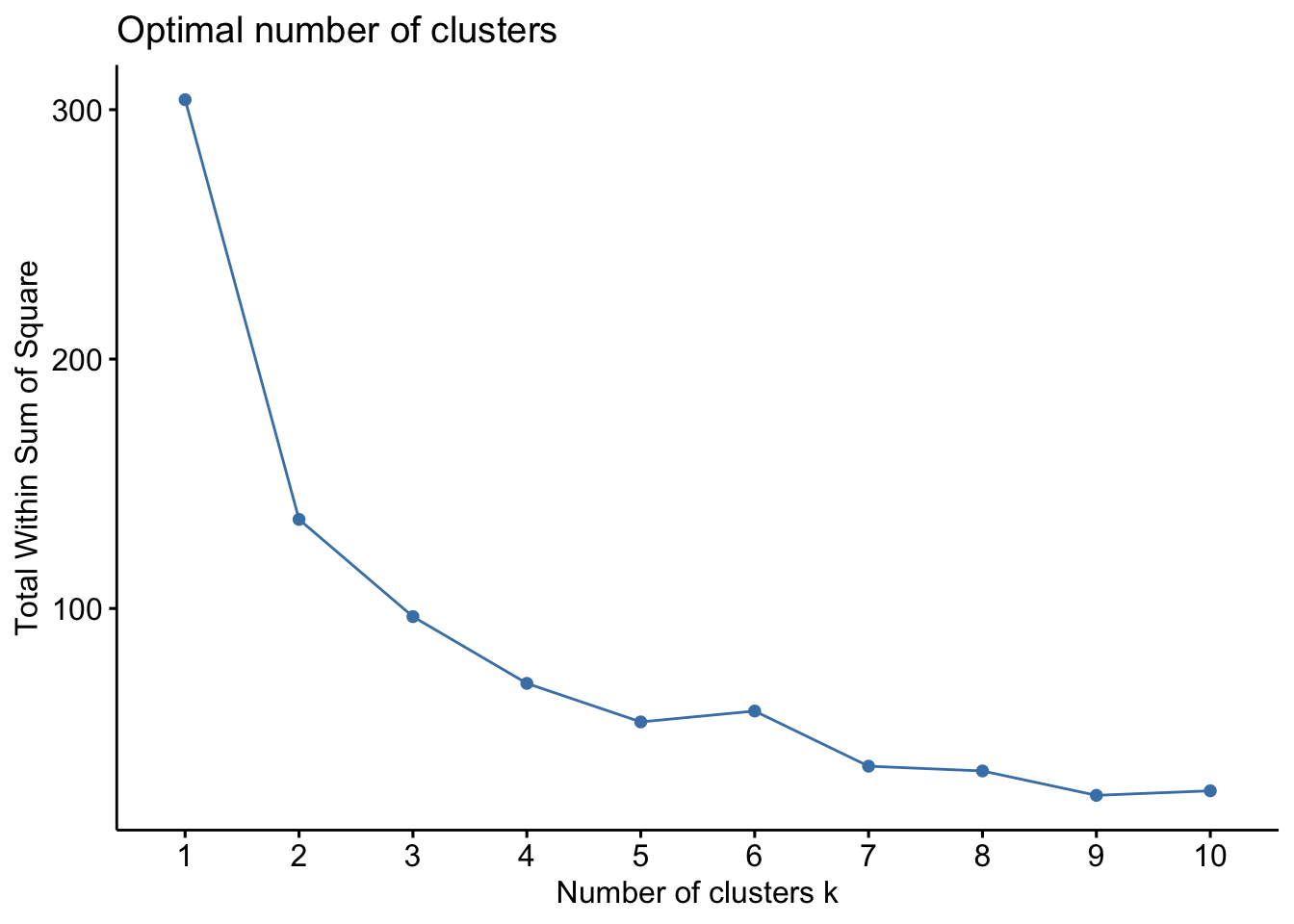
When we increase the number of cluster the total wss will get smaller and smaller (but obviously from an interpretability point of view we would like to have a reduced number of groups). We try to identify in the plot an elbow. We see for example that after 5 cluster we have an increase in the total wss. This is a good suggestion to use 5 clusters.
set.seed(44)
cl5 = kmeans(scaledevnum,
            centers = 5, #n. of clusters
            iter.max = 1000,
            nstart = 25) #run the alg. 25 times

autoplot(cl5,
         data = scaledevnum,
         scale = 0,#scaled data
         label = TRUE,
         frame = TRUE,
         frame.type = "norm")
## Too few points to calculate an ellipse
## Too few points to calculate an ellipse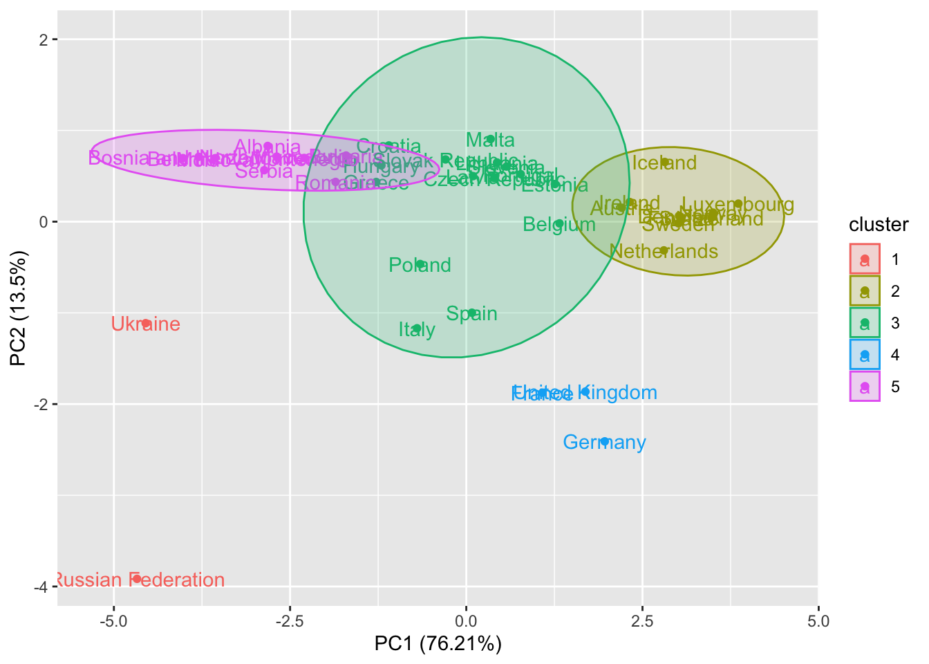
For two clusters which are very small (the red and the blue) it is not possible to draw the ellipse.
9.3 Exercises Lab 8
The RMarkdown file Lab7_home_exercises_empty.Rmd contains the exercise for Lab. 7. Write your solutions in the RMarkdown file and produce the final html file containing your code, your comments and all the outputs.