Chapter 7 R Lab 6 - 26/05/2021
In this lecture we will learn how to implement support vector machine, and we will compare its version with other classification algorithms. In this lecture we will learn how to implement the Adaboost algorithm and support vector machines.
The following packages are required: MASS,e1071, pROC, randomForest and tidyverse.
library(MASS) #for LDA and QDA
library(tidyverse)
library(e1071) #for SVM
library(pROC)
For this lab sesion the simulated data contained in the file simdata.rds will be used (the file is available in the e-learning). The extension .rds refers to a format which is specific to R software. The file contains a R object which can be restored by using the function readRDS.
#Easy way: the RDS file must be in the same folder of the Rmd file
simdata = readRDS("/Users/marco/Google Drive Personale/Formazione/3_Unibg/2021-22/ML_tutor/RLabs/Lab6/simdata.rds")
glimpse(simdata)
## Rows: 200
## Columns: 3
## $ x.1 <dbl> 1.8735462, 2.6836433, 1.6643714, 4.0952808, 2.8295078, 1.6795316, …
## $ x.2 <dbl> 2.9094018, 4.1888733, 4.0865884, 2.1690922, 0.2147645, 4.9976616, …
## $ y <dbl> 1, 1, 1, 1, 1, 1, 1, 1, 1, 1, 1, 1, 1, 1, 1, 1, 1, 1, 1, 1, 1, 1, …The simulated data contains two regressors and the response variable y which we now transform into a factor with labels -1 and +1.
table(simdata$y)##
## 1 2
## 150 50simdata$y = factor(simdata$y, labels=c(-1,+1))
table(simdata$y)##
## -1 1
## 150 50We also plot the data (scatterplot) by placing x.1 and x.2 on the x and y axis, and by using the categories of the response variable y for setting the color of the points.
simdata %>%
  ggplot() +
  geom_point(aes(x.1, x.2, col=y))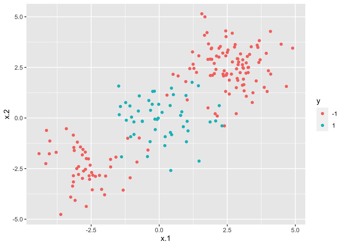
From the plot it results that the data can’t be separated by a linear decision boundary.
As usual, we split the data into a training and a test set. The first one, named simdata_tr, contains 70% of the observations. The latter is named simdata_te.
set.seed(4,sample.kind = "Rejection")
index = sample(1:nrow(simdata),0.7*nrow(simdata))
simdata_tr = simdata[index,]
simdata_te = simdata[-index,]
We can conclude that …..
7.1 SVM
We use the same data (simdata_tr and simdata_te) to implement SVM by using the function svm contained in the e1071 library (see ?svm). In particular, given the structure of the data a linear kernel won’t be taken into account; we will use instead a radial kernel and polynomal kernel.
We start by implement SVM with a polynomial kernel with \(degree=4\) and cost parameter \(C=1\).
svmfit.poly <- svm(y~.,
                   data= simdata_tr,
                   kernel = "polynomial",
                   cost = 1,
                   degree = 4,
                   scale = T)
From the output we see that there are 66 training observations classified as support vectors. We can now use the function plot.svm to represent graphically the output (see ?plot.svm).
plot(svmfit.poly, simdata_tr, grid=200)# grid improve the resolution of the plot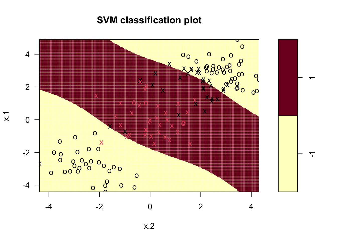 In the figure we see the training observations represented by different colors: red symbols belong to the category +1, while black symbols to the category -1. Crosses (instead of circles) are used to denote the support vectors. Finally the background color represents the predicted category: the red area defines the values of the regressors for which the prediction of
 y is equal to +1. Elsewhere (in the yellow area) the prediction will be given by category -1. The option grid of the plot function improves the resolution of the prediction areas (the higher the value, the higher the resolution).
As usual, we compute predictions and then the accuracy.
# pred with polynomial
svmfit.poly_pred <- predict(svmfit.poly, newdata=simdata_te)
# cf
table(svmfit.poly_pred,simdata_te$y)
##
## svmfit.poly_pred -1 1
## -1 40 2
## 1 7 11# accuracy
mean(svmfit.poly_pred == simdata_te$y)## [1] 0.85Let’s train the svm algorithm also for the radial kernel. In this case, we will set the following parameters: \(cost=1\) and \(gamma=1\)
svmfit.radial <- svm(y~.,
                     data=simdata_tr,
                     kernel = "radial",
                     gamma = 1,
                     cost = 1,
                     scale= T)
Let’s visualize what’s going on:
plot(svmfit.radial,simdata_tr, grid=200)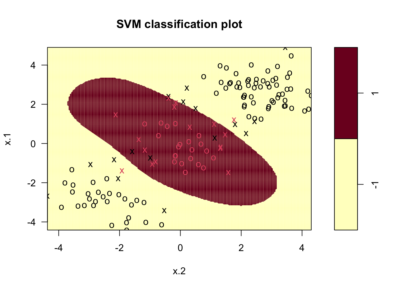
As we did before, we can evaluate our results using the confusion matrix and the accuracy. In order to do that, we need the final prediction.
# pred with radial
svmfit.radial_pred <- predict(svmfit.radial, newdata=simdata_te)
# cf
table(svmfit.radial_pred,simdata_te$y)
##
## svmfit.radial_pred -1 1
## -1 45 2
## 1 2 11# accuracy
mean(svmfit.radial_pred == simdata_te$y)## [1] 0.9333333Let’s now change the value of \(\gamma\) to 2 (\(\gamma >0\)) and keep \(C=1\). How does the accuracy change?
svmfit.radial_2 = svm(y~.,
           data = simdata_tr,
           kernel = "radial",
           cost = 1,
           gamma = 2,
           scale= T)
#predictions
svmfit.radial_2_pred = predict(svmfit.radial_2, newdata=simdata_te)
#matrix
table(svmfit.radial_2_pred, simdata_te$y)
##
## svmfit.radial_2_pred -1 1
## -1 45 3
## 1 2 10#accuracy
mean(svmfit.radial_2_pred == simdata_te$y)## [1] 0.9166667By changing the value of \(\gamma\) the accuracy decreases slightly.
Let’s now consider different parameters for both the radial (\(C\) and \(\gamma\)) and the polynomial (\(degree\) and \(C\)) kernel and see which is the best combination in terms of cross-validation accuracy. In this case, instead of proceeding with a for loop as described in the last lab, we will use the function tune implemented in the e1071 library. Given that we use CV we set the seed equal to 1. In particular, we consider for \(C\) the values cost=c(0.1,1,10,100,1000), for \(\gamma\) the integers from 1 to 10 (1:10 or seq(1,10)) and for \(degree\) the integer values from 4 to 8).
# radial tuning
set.seed(1,sample.kind = "Rejection")
tune.svm.radial = tune(svm, #function to run iteratively
                y ~ .,
                data = simdata_tr,
                kernel = "radial",
                ranges = list(cost = c(0.1,1,10,100,1000),
                              gamma = 1:10))
By typing
summary(tune.svm.radial)##
## Parameter tuning of 'svm':
##
## - sampling method: 10-fold cross validation
##
## - best parameters:
## cost gamma
## 0.1 1
##
## - best performance: 0.05714286
##
## - Detailed performance results:
## cost gamma error dispersion
## 1 1e-01 1 0.05714286 0.05634362
## 2 1e+00 1 0.06428571 0.07103064
## 3 1e+01 1 0.08571429 0.06563833
## 4 1e+02 1 0.09285714 0.06776309
## 5 1e+03 1 0.07142857 0.05832118
## 6 1e-01 2 0.08571429 0.06563833
## 7 1e+00 2 0.07142857 0.06734350
## 8 1e+01 2 0.08571429 0.05634362
## 9 1e+02 2 0.08571429 0.06563833
## 10 1e+03 2 0.10000000 0.07678341
## 11 1e-01 3 0.11428571 0.09035079
## 12 1e+00 3 0.07142857 0.06734350
## 13 1e+01 3 0.07857143 0.05270463
## 14 1e+02 3 0.07857143 0.06254250
## 15 1e+03 3 0.10000000 0.07678341
## 16 1e-01 4 0.15000000 0.09190600
## 17 1e+00 4 0.07857143 0.06254250
## 18 1e+01 4 0.07857143 0.05270463
## 19 1e+02 4 0.08571429 0.07377111
## 20 1e+03 4 0.10714286 0.10780220
## 21 1e-01 5 0.16428571 0.09553525
## 22 1e+00 5 0.08571429 0.08109232
## 23 1e+01 5 0.10000000 0.06023386
## 24 1e+02 5 0.09285714 0.08940468
## 25 1e+03 5 0.10000000 0.09642122
## 26 1e-01 6 0.20714286 0.10350983
## 27 1e+00 6 0.07857143 0.06254250
## 28 1e+01 6 0.10000000 0.06023386
## 29 1e+02 6 0.10000000 0.09642122
## 30 1e+03 6 0.10714286 0.09066397
## 31 1e-01 7 0.25000000 0.08417938
## 32 1e+00 7 0.09285714 0.06776309
## 33 1e+01 7 0.09285714 0.06776309
## 34 1e+02 7 0.10714286 0.09066397
## 35 1e+03 7 0.10714286 0.09066397
## 36 1e-01 8 0.26428571 0.10129546
## 37 1e+00 8 0.10000000 0.06900656
## 38 1e+01 8 0.10000000 0.07678341
## 39 1e+02 8 0.10714286 0.09066397
## 40 1e+03 8 0.10714286 0.09066397
## 41 1e-01 9 0.26428571 0.10129546
## 42 1e+00 9 0.10000000 0.06900656
## 43 1e+01 9 0.10000000 0.07678341
## 44 1e+02 9 0.10714286 0.09066397
## 45 1e+03 9 0.10714286 0.09066397
## 46 1e-01 10 0.26428571 0.10129546
## 47 1e+00 10 0.10714286 0.06941609
## 48 1e+01 10 0.10714286 0.08417938
## 49 1e+02 10 0.11428571 0.09642122
## 50 1e+03 10 0.11428571 0.09642122we obtain a data frame with 50 rows (one for each hyperparameter combination). We are interested in the third column (error) giving us the cross-validation error for a specific value of cost and gamma. In particular, we look for the value of \(C\) and \(\gamma\) for which error is lowest. This information is provided automatically in the ouput of tune. In fact the object tune.svm (it’s a list) contains the following objects:
names(tune.svm.radial)## [1] "best.parameters" "best.performance" "method" "nparcomb"
## [5] "train.ind" "sampling" "performances" "best.model"By using the $ we can extract the best combination of parameters ($best.parameters), the corresponding cv error ($best.performance) and the corresponding estimate svm model ($best.model):
tune.svm.radial$best.parameters## cost gamma
## 1 0.1 1tune.svm.radial$best.performance #cv error## [1] 0.05714286tune.svm.radial$best.model##
## Call:
## best.tune(method = svm, train.x = y ~ ., data = simdata_tr, ranges = list(cost = c(0.1,
## 1, 10, 100, 1000), gamma = 1:10), kernel = "radial")
##
##
## Parameters:
## SVM-Type: C-classification
## SVM-Kernel: radial
## cost: 0.1
##
## Number of Support Vectors: 72If you are interest in computing class predictions for the test observation given the best hyperparameter setting, you could use the object tune.svm$best.model directly in the predict function.
Let’s tune also the polynomial kernel. A computation error will be displayed related to the number of interation. This is due to a limit of the e1071 package, but still the results are pretty good.
tune.svm.poly <- tune(svm,
                      y ~.,
                      data= simdata_tr,
                      kernel = "polynomial",
                      ranges = list(cost = c(0.1,1,10,100,1000),
                                    degree = 4:8))
As we did before, we can check our results:
summary(tune.svm.poly)##
## Parameter tuning of 'svm':
##
## - sampling method: 10-fold cross validation
##
## - best parameters:
## cost degree
## 10 4
##
## - best performance: 0.1214286
##
## - Detailed performance results:
## cost degree error dispersion
## 1 1e-01 4 0.2642857 0.11688512
## 2 1e+00 4 0.1642857 0.10129546
## 3 1e+01 4 0.1214286 0.10129546
## 4 1e+02 4 0.1285714 0.11065667
## 5 1e+03 4 0.1357143 0.12348860
## 6 1e-01 5 0.2642857 0.11688512
## 7 1e+00 5 0.2642857 0.11688512
## 8 1e+01 5 0.2642857 0.11688512
## 9 1e+02 5 0.2642857 0.11688512
## 10 1e+03 5 0.2642857 0.11688512
## 11 1e-01 6 0.2642857 0.11688512
## 12 1e+00 6 0.2642857 0.13062730
## 13 1e+01 6 0.1428571 0.10101525
## 14 1e+02 6 0.1500000 0.10884885
## 15 1e+03 6 0.1428571 0.11167657
## 16 1e-01 7 0.2642857 0.11688512
## 17 1e+00 7 0.2642857 0.11688512
## 18 1e+01 7 0.2642857 0.11688512
## 19 1e+02 7 0.2714286 0.12046772
## 20 1e+03 7 0.2785714 0.13656791
## 21 1e-01 8 0.2642857 0.11688512
## 22 1e+00 8 0.3142857 0.09642122
## 23 1e+01 8 0.2000000 0.12953781
## 24 1e+02 8 0.1500000 0.09788002
## 25 1e+03 8 0.1428571 0.11664237Besides class predictions we also need probabilities in order to compute the ROC curve. In the case of svm, probabilities are a transformation of the decision values (the latter is the computed values of the hyperplane equation). To obtain this additional information we will use the options decision.values = T,probability = T in the svm and predict functions (run with the best parameter setting). We start with the polynomial kernel:
set.seed(4, sample.kind="Rejection")
best.svm.poly <- svm(y~.,
                     data= simdata_tr,
                     kernel = "polynomial",
                     cost = tune.svm.poly$best.model$cost,
                     degree = tune.svm.poly$best.model$degree,
                     decision.values = T,
                     probability = T)
best.svm.poly
##
## Call:
## svm(formula = y ~ ., data = simdata_tr, kernel = "polynomial", cost = tune.svm.poly$best.model$cost,
## degree = tune.svm.poly$best.model$degree, decision.values = T,
## probability = T)
##
##
## Parameters:
## SVM-Type: C-classification
## SVM-Kernel: polynomial
## cost: 10
## degree: 4
## coef.0: 0
##
## Number of Support Vectors: 47# compute predictions + decision.values + probabilities for the test set
best.svm.poly_pred <- predict(best.svm.poly,
newdata = simdata_te,
decision.values = T,
probability = T)
# accuracy
mean(best.svm.poly_pred == simdata_te$y)## [1] 0.9And then we compute the same for the radial kernel:
set.seed(4, sample.kind="Rejection")
best.svm.radial <- svm(y~.,
                       data = simdata_tr,
                       kernel = "radial",
                       cost = tune.svm.radial$best.model$cost,
                       gamma = tune.svm.radial$best.model$gamma,
                       decision.values = T,
                       probability = T)
### predictions ----

best.svm.radial_pred <- predict(best.svm.radial,
                                newdata= simdata_te,
                                decision.values = T,
                                probability = T)

best.svm.radial_pred
## 4 6 15 16 17 18 20 23 27 28 29 30 34 38 40 42 58 66 67 69
## -1 -1 -1 -1 -1 -1 -1 -1 -1 1 -1 -1 -1 -1 -1 -1 -1 -1 -1 -1
## 70 74 77 81 83 89 93 94 95 96 97 100 104 105 108 111 118 120 122 123
## -1 -1 1 -1 -1 -1 -1 -1 -1 -1 -1 -1 -1 -1 -1 -1 -1 -1 1 -1
## 127 131 132 135 137 138 145 161 166 167 168 169 173 174 177 183 185 189 195 197
## -1 -1 -1 -1 -1 -1 -1 -1 -1 1 1 1 1 1 1 1 1 1 1 -1
## attr(,"decision.values")
## -1/1
## 4 1.06518441
## 6 0.84167159
## 15 1.06858105
## 16 1.05818023
## 17 1.12076184
## 18 1.00155250
## 20 1.18328236
## 23 1.05891038
## 27 1.09073903
## 28 -0.24029197
## 29 1.12672134
## 30 1.19500107
## 34 1.18629143
## 38 0.82583782
## 40 1.17505398
## 42 1.13874828
## 58 1.04362613
## 66 1.19715857
## 67 0.35795172
## 69 1.13898919
## 70 0.93318949
## 74 0.80881534
## 77 0.12955352
## 81 1.13100955
## 83 1.01380301
## 89 1.19192259
## 93 1.12976497
## 94 0.93421936
## 95 0.90326506
## 96 1.18955055
## 97 1.00085098
## 100 1.01855088
## 104 1.10251370
## 105 0.77933440
## 108 0.58175356
## 111 0.97148119
## 118 1.12755593
## 120 1.01506129
## 122 -0.28235461
## 123 0.92997806
## 127 1.12436155
## 131 1.11028940
## 132 0.98968024
## 135 1.07647966
## 137 0.91201312
## 138 1.13258450
## 145 0.82162717
## 161 0.23441855
## 166 0.39336978
## 167 -0.95681700
## 168 -0.72181341
## 169 -0.91335816
## 173 -0.77448799
## 174 -1.04954849
## 177 -0.74116942
## 183 -0.75257449
## 185 -0.39323003
## 189 0.04169849
## 195 -0.74245356
## 197 0.47814541
## attr(,"probabilities")
## -1 1
## 4 0.975646242 0.02435376
## 6 0.943066454 0.05693355
## 15 0.975963108 0.02403689
## 16 0.974979925 0.02502007
## 17 0.980353536 0.01964646
## 18 0.968900987 0.03109901
## 20 0.984587623 0.01541238
## 23 0.975050207 0.02494979
## 27 0.977933636 0.02206636
## 28 0.187263584 0.81273642
## 29 0.980801982 0.01919802
## 30 0.985274737 0.01472526
## 34 0.984767012 0.01523299
## 38 0.939612664 0.06038734
## 40 0.984086397 0.01591360
## 42 0.981676643 0.01832336
## 58 0.973538101 0.02646190
## 66 0.985397910 0.01460209
## 67 0.710114260 0.28988574
## 69 0.981693757 0.01830624
## 70 0.959645650 0.04035435
## 74 0.935681493 0.06431851
## 77 0.498368417 0.50163158
## 81 0.981118442 0.01888156
## 83 0.970326884 0.02967312
## 89 0.985097212 0.01490279
## 93 0.981027125 0.01897287
## 94 0.959802943 0.04019706
## 95 0.954809507 0.04519049
## 96 0.984958988 0.01504101
## 97 0.968817356 0.03118264
## 100 0.970862298 0.02913770
## 104 0.978915608 0.02108439
## 105 0.928305062 0.07169494
## 108 0.855726857 0.14427314
## 111 0.965114187 0.03488581
## 118 0.980863978 0.01913602
## 120 0.970469701 0.02953030
## 122 0.163270708 0.83672929
## 123 0.959151371 0.04084863
## 127 0.980625624 0.01937438
## 131 0.979540502 0.02045950
## 132 0.967455962 0.03254404
## 135 0.976684484 0.02331552
## 137 0.956277745 0.04372226
## 138 0.981233380 0.01876662
## 145 0.938661711 0.06133829
## 161 0.600566194 0.39943381
## 166 0.738055375 0.26194463
## 167 0.013399059 0.98660094
## 168 0.033229727 0.96677027
## 169 0.015869444 0.98413056
## 173 0.027155409 0.97284459
## 174 0.009326832 0.99067317
## 177 0.030858540 0.96914146
## 183 0.029538946 0.97046105
## 185 0.111829247 0.88817075
## 189 0.412493654 0.58750635
## 195 0.030707157 0.96929284
## 197 0.797518746 0.20248125
## Levels: -1 1# accuracy
mean(best.svm.radial_pred == simdata_te$y)## [1] 0.9By typing best.svm.radial_pred or attributes(best.svm.radial_pred) we see that the object best.svm.radial_pred contains more information than just the predicted categories. The same applies also to the polynomial predictions. We are in particular interested in the attribute called "probabilities" which can be extracted as follows:
best.svm.poly_prob <- attr(best.svm.poly_pred, "probabilities")
best.svm.radial_prob <- attr(best.svm.radial_pred, "probabilities")
We are now able to compute and plot the ROC curve as described in Section ??:
library(pROC)
rocsvm.poly <- roc(simdata_te$y,best.svm.poly_prob[,1])
## Setting levels: control = -1, case = 1## Setting direction: controls > casesrocsvm.radial <- roc(simdata_te$y, best.svm.radial_prob[,1])## Setting levels: control = -1, case = 1
## Setting direction: controls > casesggroc(list(poly = rocsvm.poly,
radial = rocsvm.radial))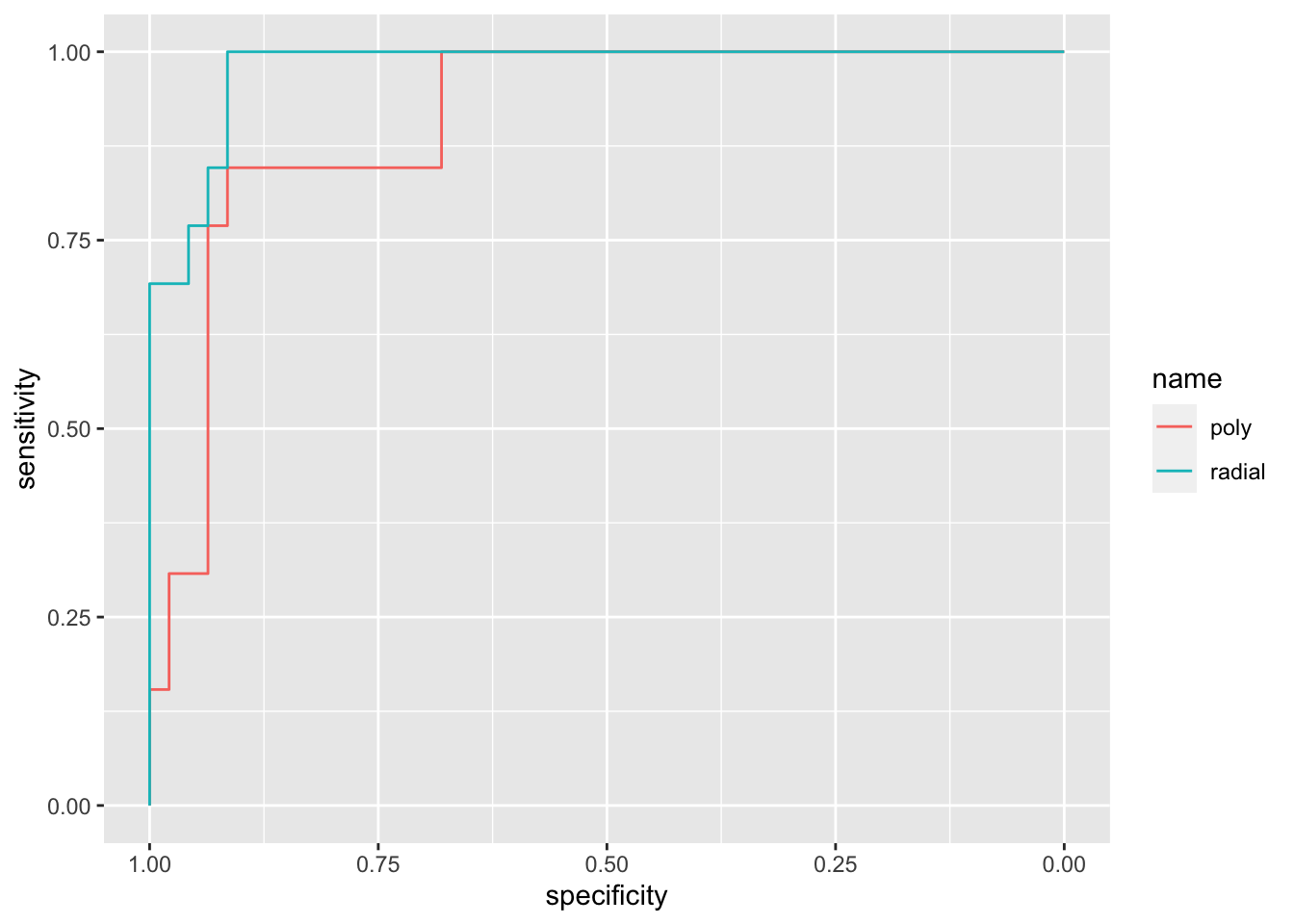
# comparing between them, radial seems better.
auc(rocsvm.poly)
## Area under the curve: 0.9116auc(rocsvm.radial)## Area under the curve: 0.9787What can we conclude? Well, considering that both the tuned algorithms are obtaining an accuracy equal to 0.9, we should consider the AUC in order to discriminate between them. In fact, take into consideration that AUC check sensitivity e specificity (so two “tests”) for several scenarios, while the accuracy consider just the missclassified observation in the best scenario. With this respect, I would go for radial kernel!
7.2 COMPARISON WITH QDA AND BAGGING
We compare, by means of accuracy, the svm algorithm with quadratic discriminant analysis (QDA) and bagging algorithm.
## QDA -----
library(MASS)
set.seed(1, sample.kind="Rejection")
qda_simdata <- qda(y~.,
                   data= simdata_tr)

pred_qda <- predict(qda_simdata, newdata= simdata_te)

#cf
table(pred_qda$class, simdata_te$y)
##
## -1 1
## -1 47 6
## 1 0 7#accuracy
mean(pred_qda$class == simdata_te$y)## [1] 0.9rocqda <- roc(simdata_te$y, pred_qda$posterior[,1])## Setting levels: control = -1, case = 1## Setting direction: controls > cases## BAGGING -----
library(randomForest) #for bagging+RF
set.seed(1, sample.kind="Rejection")
bag_fit <- randomForest(formula = y~.,
data= simdata_tr,
importance = T,
ntree = 500,
mtry = ncol(simdata_tr)-1)
bag_fit_prob <- predict(bag_fit,
newdata= simdata_te,
type = "prob")
bag_fit_class <- predict(bag_fit,
newdata= simdata_te,
type = "class")
# cf
table(bag_fit_class, simdata_te$y)##
## bag_fit_class -1 1
## -1 45 4
## 1 2 9# accuracy
mean(bag_fit_class == simdata_te$y)## [1] 0.9rocbag <- roc(simdata_te$y, bag_fit_prob[,1])## Setting levels: control = -1, case = 1## Setting direction: controls > casesFinally, we can evaluate everything togheter:
ggroc(list(svm.poly = rocsvm.poly,
           svm.radial = rocsvm.radial,
           qda = rocqda,
bagging = rocbag)) %>% plotly::ggplotly()auc(rocbag)## Area under the curve: 0.9722auc(rocqda)## Area under the curve: 0.982auc(rocsvm.radial)## Area under the curve: 0.9787auc(rocsvm.poly)## Area under the curve: 0.9116As we already know, svm with polynomial kernel performe worse than its radial counterpart. At the same time, both QDA and Bagging seems to reach a good results. In this case, we should take into consideration not only the AUC and the accuracy, but also the algorithm characteristics as:
- Stability of decision
- Computational requirements
- Interpretability
Also, take into consideration that we didn’t tune any parameter of QDA and Bagging. If we just want to remain on a basic interpretation, QDA should be preferred. But real-life problems are not always requiring a basic interpretation!
7.3 SVM with more than 2 categories and more than 2 regressors
We consider now the Glass dataset contained in the mlbench library (see ?Glass). We start by exploring the data where Type is the response variale.
library(mlbench)
data(Glass)
glimpse(Glass)
## Rows: 214
## Columns: 10
## $ RI <dbl> 1.52101, 1.51761, 1.51618, 1.51766, 1.51742, 1.51596, 1.51743, 1.…
## $ Na <dbl> 13.64, 13.89, 13.53, 13.21, 13.27, 12.79, 13.30, 13.15, 14.04, 13…
## $ Mg <dbl> 4.49, 3.60, 3.55, 3.69, 3.62, 3.61, 3.60, 3.61, 3.58, 3.60, 3.46,…
## $ Al <dbl> 1.10, 1.36, 1.54, 1.29, 1.24, 1.62, 1.14, 1.05, 1.37, 1.36, 1.56,…
## $ Si <dbl> 71.78, 72.73, 72.99, 72.61, 73.08, 72.97, 73.09, 73.24, 72.08, 72…
## $ K <dbl> 0.06, 0.48, 0.39, 0.57, 0.55, 0.64, 0.58, 0.57, 0.56, 0.57, 0.67,…
## $ Ca <dbl> 8.75, 7.83, 7.78, 8.22, 8.07, 8.07, 8.17, 8.24, 8.30, 8.40, 8.09,…
## $ Ba <dbl> 0, 0, 0, 0, 0, 0, 0, 0, 0, 0, 0, 0, 0, 0, 0, 0, 0, 0, 0, 0, 0, 0,…
## $ Fe <dbl> 0.00, 0.00, 0.00, 0.00, 0.00, 0.26, 0.00, 0.00, 0.00, 0.11, 0.24,…
## $ Type <fct> 1, 1, 1, 1, 1, 1, 1, 1, 1, 1, 1, 1, 1, 1, 1, 1, 1, 1, 1, 1, 1, 1,…We see that the response variable is characterized by 6 categories:
table(Glass$Type)##
## 1 2 3 5 6 7
## 70 76 17 13 9 29We proceed with some descriptive plotting:
Glass %>%
  ggplot()+
  geom_point(aes(RI,Na,col=Type))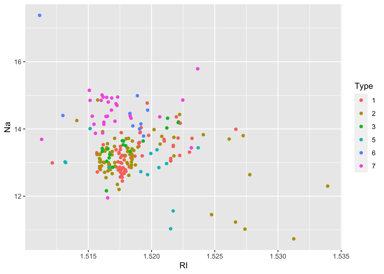
Glass %>%
  ggplot()+
  geom_boxplot(aes(Mg,fill=Type))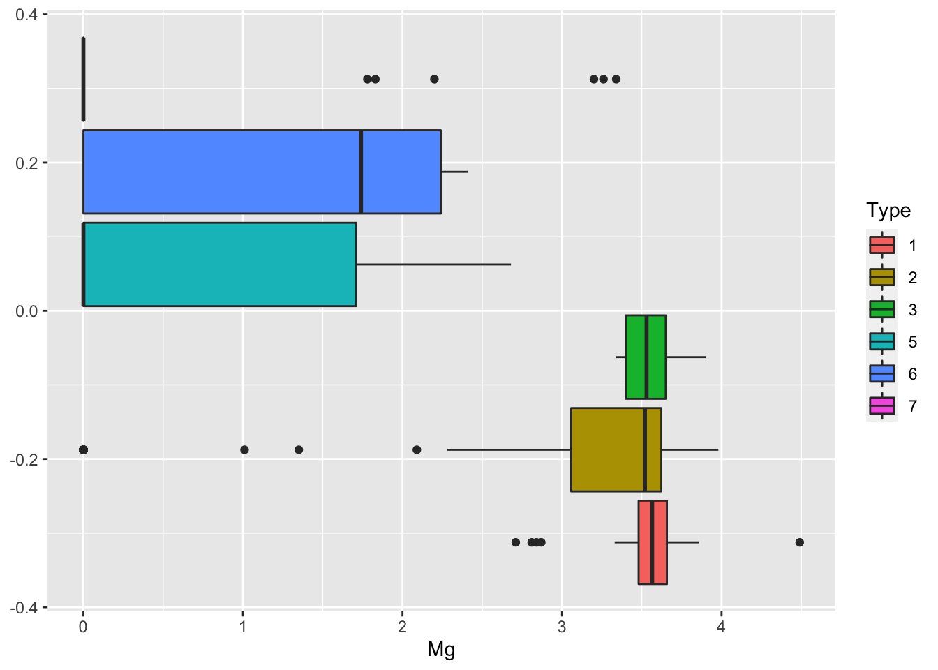
We then create as usual the training (70%) and test data set.
set.seed(44,sample.kind = "Rejection")
tr_index = sample(1:nrow(Glass), nrow(Glass)*0.7)
Glass_tr = Glass[tr_index,]
Glass_te = Glass[-tr_index,]
Finally, we implement SVM. Note that the function svm uses the one-against-one approach. We consider in this case a polynomial kernel of degree \(d\) 1 and a value of \(C=1\). We then compute predictions and accuracy.
svm.fit = svm(Type ~ .,
              data = Glass_tr,
              kernel = "polynomial",
              cost = 1,
              degree = 1)
svm.pred = predict(svm.fit,
                   Glass_te)

table(svm.pred, Glass_te$Type)
##
## svm.pred 1 2 3 5 6 7
## 1 21 11 2 0 0 0
## 2 2 12 1 2 0 0
## 3 0 0 0 0 0 0
## 5 0 1 0 0 0 0
## 6 0 2 0 0 0 0
## 7 0 1 0 3 0 7mean(svm.pred == Glass_te$Type)## [1] 0.6153846To tune the hyperparameters we consider different values of \(C\) (cost=c(0.1,1,10,100,1000)) and of the degree of the polynomial(1:5) and then compute the accuracy for each combination of hyperparameters.
set.seed(1,sample.kind = "Rejection")
tune.out=tune(svm,
              Type ~ .,
              data = Glass_tr,
              kernel="polynomial",
              ranges=list(cost=c(0.1,1,10,100,1000),
                          degree=1:5))
summary(tune.out)
##
## Parameter tuning of 'svm':
##
## - sampling method: 10-fold cross validation
##
## - best parameters:
## cost degree
## 1000 3
##
## - best performance: 0.3142857
##
## - Detailed performance results:
## cost degree error dispersion
## 1 1e-01 1 0.5838095 0.07566619
## 2 1e+00 1 0.3952381 0.11306669
## 3 1e+01 1 0.3542857 0.10697989
## 4 1e+02 1 0.3209524 0.11070675
## 5 1e+03 1 0.3347619 0.10228062
## 6 1e-01 2 0.5966667 0.07445274
## 7 1e+00 2 0.5095238 0.09735737
## 8 1e+01 2 0.3747619 0.18767853
## 9 1e+02 2 0.3147619 0.13592437
## 10 1e+03 2 0.3480952 0.17874524
## 11 1e-01 3 0.6104762 0.07005019
## 12 1e+00 3 0.5300000 0.09993825
## 13 1e+01 3 0.3614286 0.12051895
## 14 1e+02 3 0.3547619 0.15259988
## 15 1e+03 3 0.3142857 0.12832624
## 16 1e-01 4 0.5761905 0.10021393
## 17 1e+00 4 0.5566667 0.10189561
## 18 1e+01 4 0.4890476 0.10079178
## 19 1e+02 4 0.3619048 0.13997084
## 20 1e+03 4 0.3347619 0.12801270
## 21 1e-01 5 0.5685714 0.13333711
## 22 1e+00 5 0.5566667 0.09692813
## 23 1e+01 5 0.5100000 0.11764143
## 24 1e+02 5 0.4561905 0.09706709
## 25 1e+03 5 0.3890476 0.13903258tune.out$best.parameters## cost degree
## 15 1000 3# prediction (based on the one-versus-one approach)
svm.pred.best = predict(tune.out$best.model,
newdata=Glass_te)
table(svm.pred.best, Glass_te$Type)##
## svm.pred.best 1 2 3 5 6 7
## 1 19 4 2 1 0 0
## 2 2 17 0 3 0 1
## 3 2 2 1 0 0 0
## 5 0 1 0 0 0 0
## 6 0 2 0 0 0 0
## 7 0 1 0 1 0 6mean(svm.pred.best == Glass_te$Type)## [1] 0.6615385Note that in this case the confusion matrix is not a 2 by 2 matrix, but it’s dimension is given by the number of categories of the response variable.
7.4 Exercises Lab 6
The RMarkdown file Lab6_home_exercises_empty.Rmd contains the exercise for Lab 6. Write your solutions in the RMarkdown file and produce the final html file containing your code, your comments and all the outputs.