Chapter 2 R Lab 1 - 17/03/2021
In this lecture we will learn how to implement the K-nearest neighbors (KNN) method for classification and regression problems.
The following packages are required: class, FNN and tidyverse.
library(class)
library(FNN)
##
## Attaching package: 'FNN'## The following objects are masked from 'package:class':
##
## knn, knn.cvlibrary(tidyverse)## ── Attaching packages ─────────────────────────────────────── tidyverse 1.3.1 ──## ✓ ggplot2 3.3.5 ✓ purrr 0.3.4
## ✓ tibble 3.1.6 ✓ dplyr 1.0.7
## ✓ tidyr 1.1.4 ✓ stringr 1.4.0
## ✓ readr 2.1.2 ✓ forcats 0.5.1## Warning: package 'readr' was built under R version 4.0.5## ── Conflicts ────────────────────────────────────────── tidyverse_conflicts() ──
## x dplyr::filter() masks stats::filter()
## x dplyr::lag() masks stats::lag()library(plotly)##
## Attaching package: 'plotly'## The following object is masked from 'package:ggplot2':
##
## last_plot## The following object is masked from 'package:stats':
##
## filter## The following object is masked from 'package:graphics':
##
## layout2.1 KNN for regression problems
For KNN regression we will use data regarding bike sharing (link). The data are stored in the file named bikesharing.csv which is available in the e-learning. The data regard the bike sharing counts aggregated on daily basis.
We start by importing the data. Please, note that in the following code my file path is shown; obviously for your computer it will be different:
bike = read.csv("/Users/marco/Google Drive Personale/Formazione/3_Unibg/2021-22/ML_tutor/RLabs/Lab1/bikesharing.csv")
head(bike)
## instant dteday season yr mnth holiday weekday workingday weathersit
## 1 1 2011-01-01 1 0 1 0 6 0 2
## 2 2 2011-01-02 1 0 1 0 0 0 2
## 3 3 2011-01-03 1 0 1 0 1 1 1
## 4 4 2011-01-04 1 0 1 0 2 1 1
## 5 5 2011-01-05 1 0 1 0 3 1 1
## 6 6 2011-01-06 1 0 1 0 4 1 1
## temp atemp hum windspeed casual registered cnt
## 1 0.344167 0.363625 0.805833 0.1604460 331 654 985
## 2 0.363478 0.353739 0.696087 0.2485390 131 670 801
## 3 0.196364 0.189405 0.437273 0.2483090 120 1229 1349
## 4 0.200000 0.212122 0.590435 0.1602960 108 1454 1562
## 5 0.226957 0.229270 0.436957 0.1869000 82 1518 1600
## 6 0.204348 0.233209 0.518261 0.0895652 88 1518 1606glimpse(bike)## Rows: 731
## Columns: 16
## $ instant <int> 1, 2, 3, 4, 5, 6, 7, 8, 9, 10, 11, 12, 13, 14, 15, 16, 17, …
## $ dteday <chr> "2011-01-01", "2011-01-02", "2011-01-03", "2011-01-04", "20…
## $ season <int> 1, 1, 1, 1, 1, 1, 1, 1, 1, 1, 1, 1, 1, 1, 1, 1, 1, 1, 1, 1,…
## $ yr <int> 0, 0, 0, 0, 0, 0, 0, 0, 0, 0, 0, 0, 0, 0, 0, 0, 0, 0, 0, 0,…
## $ mnth <int> 1, 1, 1, 1, 1, 1, 1, 1, 1, 1, 1, 1, 1, 1, 1, 1, 1, 1, 1, 1,…
## $ holiday <int> 0, 0, 0, 0, 0, 0, 0, 0, 0, 0, 0, 0, 0, 0, 0, 0, 1, 0, 0, 0,…
## $ weekday <int> 6, 0, 1, 2, 3, 4, 5, 6, 0, 1, 2, 3, 4, 5, 6, 0, 1, 2, 3, 4,…
## $ workingday <int> 0, 0, 1, 1, 1, 1, 1, 0, 0, 1, 1, 1, 1, 1, 0, 0, 0, 1, 1, 1,…
## $ weathersit <int> 2, 2, 1, 1, 1, 1, 2, 2, 1, 1, 2, 1, 1, 1, 2, 1, 2, 2, 2, 2,…
## $ temp <dbl> 0.3441670, 0.3634780, 0.1963640, 0.2000000, 0.2269570, 0.20…
## $ atemp <dbl> 0.3636250, 0.3537390, 0.1894050, 0.2121220, 0.2292700, 0.23…
## $ hum <dbl> 0.805833, 0.696087, 0.437273, 0.590435, 0.436957, 0.518261,…
## $ windspeed <dbl> 0.1604460, 0.2485390, 0.2483090, 0.1602960, 0.1869000, 0.08…
## $ casual <int> 331, 131, 120, 108, 82, 88, 148, 68, 54, 41, 43, 25, 38, 54…
## $ registered <int> 654, 670, 1229, 1454, 1518, 1518, 1362, 891, 768, 1280, 122…
## $ cnt <int> 985, 801, 1349, 1562, 1600, 1606, 1510, 959, 822, 1321, 126…The dataset is composed by 731 rows (i.e. days) and 16 variables. We are in particular interested in the following quantitative variables (in this case \(p=3\) regressors):
atemp: normalized feeling temperature in Celsiushum: normalized humiditywindspeed: normalized wind speedcnt: count of total rental bikes (response variable)
The response variable cnt can be summarized as follows:
summary(bike$cnt)## Min. 1st Qu. Median Mean 3rd Qu. Max.
## 22 3152 4548 4504 5956 8714bike %>%
ggplot()+
geom_histogram(aes(cnt),bins=10)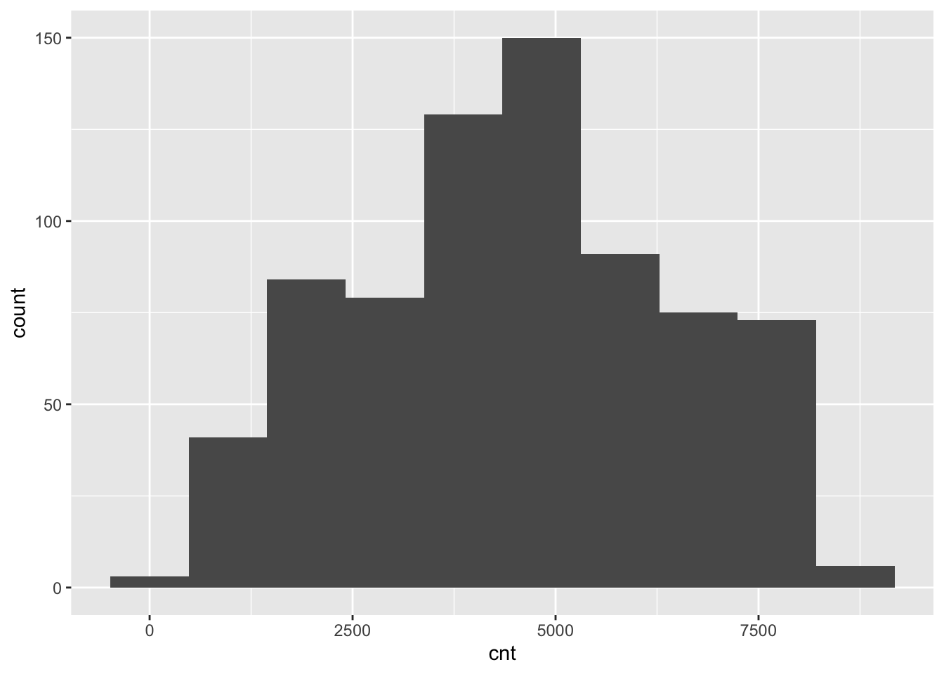
Obviously, the number of bike rentals depends strongly on weather conditions. In the following plot we represent cnt as a function of atemp and windspeed, specifying a scale color from yellow to dark blue with 12 levels:
bike %>%
  ggplot()+
  geom_point(aes(x=atemp,y=windspeed,col=cnt))+
  scale_colour_gradientn(colours = rev(hcl.colors(12)))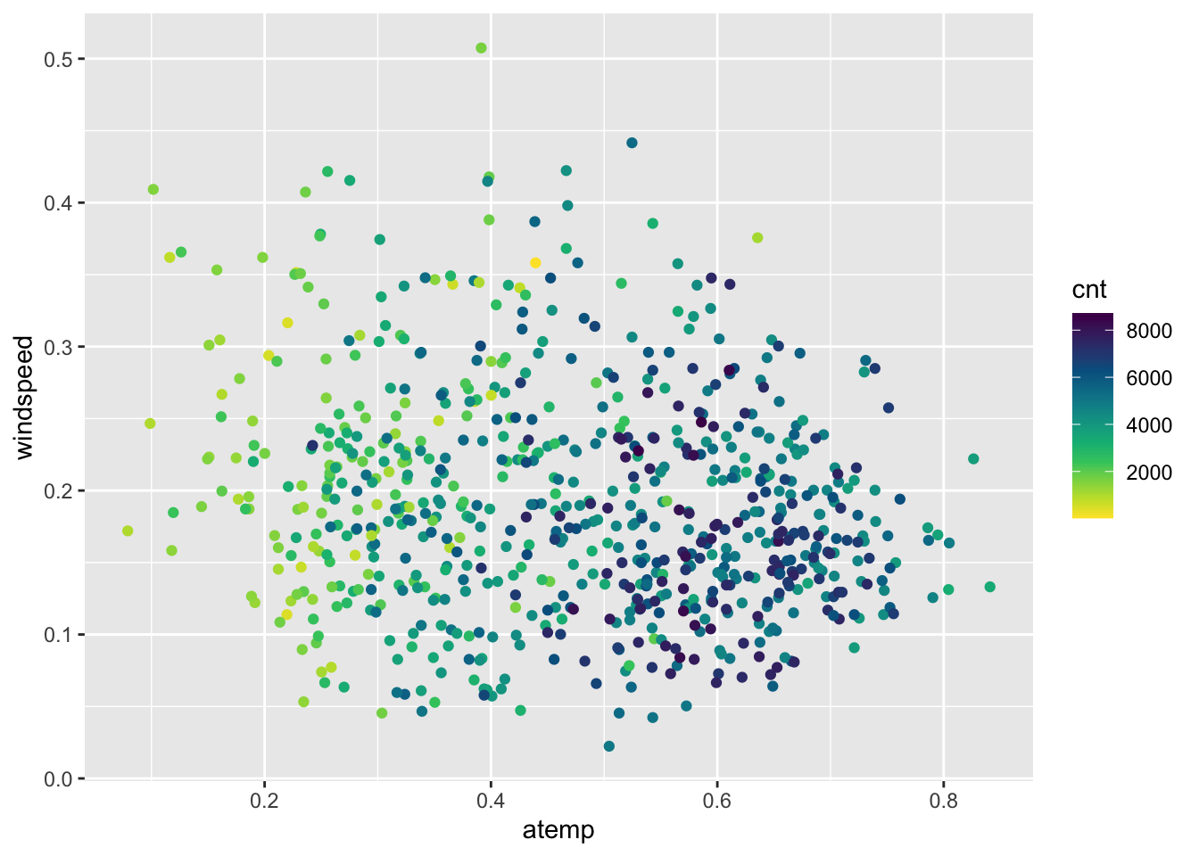
It can be observed that the number of bike rentals increases with temperature.
2.1.1 Creation of the training and testing set: method 1
We divide the dataset into 3 subsets:
- training set: containing 70% of the observations
- validating set: containing 15% of the observations
- test set: containing 15% of the observations
The procedure is done randomly by using the function sample. In order to have reproducible results, it is necessary to set the seed.
set.seed(1, sample.kind = "Rejection")
# Sample the indexes for the training observations
index <- sample(c(1,2,3),
                size=nrow(bike),
                prob=c(0.7,0.15,0.15),
                replace=T) # the same unit (1,2 or 3) must be resampled!

head(index)
## [1] 1 1 1 2 1 2# Create a new dataframe selecting the training observations
bike_training <- bike[index==1,]
head(bike_training)## instant dteday season yr mnth holiday weekday workingday weathersit
## 1 1 2011-01-01 1 0 1 0 6 0 2
## 2 2 2011-01-02 1 0 1 0 0 0 2
## 3 3 2011-01-03 1 0 1 0 1 1 1
## 5 5 2011-01-05 1 0 1 0 3 1 1
## 8 8 2011-01-08 1 0 1 0 6 0 2
## 9 9 2011-01-09 1 0 1 0 0 0 1
## temp atemp hum windspeed casual registered cnt
## 1 0.344167 0.363625 0.805833 0.160446 331 654 985
## 2 0.363478 0.353739 0.696087 0.248539 131 670 801
## 3 0.196364 0.189405 0.437273 0.248309 120 1229 1349
## 5 0.226957 0.229270 0.436957 0.186900 82 1518 1600
## 8 0.165000 0.162254 0.535833 0.266804 68 891 959
## 9 0.138333 0.116175 0.434167 0.361950 54 768 822# Create a new test dataframe selecting the validation observation
bike_validation <- bike[index==2,]
head(bike_validation)## instant dteday season yr mnth holiday weekday workingday weathersit
## 4 4 2011-01-04 1 0 1 0 2 1 1
## 6 6 2011-01-06 1 0 1 0 4 1 1
## 7 7 2011-01-07 1 0 1 0 5 1 2
## 18 18 2011-01-18 1 0 1 0 2 1 2
## 21 21 2011-01-21 1 0 1 0 5 1 1
## 29 29 2011-01-29 1 0 1 0 6 0 1
## temp atemp hum windspeed casual registered cnt
## 4 0.200000 0.212122 0.590435 0.1602960 108 1454 1562
## 6 0.204348 0.233209 0.518261 0.0895652 88 1518 1606
## 7 0.196522 0.208839 0.498696 0.1687260 148 1362 1510
## 18 0.216667 0.232333 0.861667 0.1467750 9 674 683
## 21 0.177500 0.157833 0.457083 0.3532420 75 1468 1543
## 29 0.196522 0.212126 0.651739 0.1453650 123 975 1098# Create a new test dataframe selecting the validation observation
bike_test <- bike[index==3,]
head(bike_test)## instant dteday season yr mnth holiday weekday workingday weathersit
## 15 15 2011-01-15 1 0 1 0 6 0 2
## 17 17 2011-01-17 1 0 1 1 1 0 2
## 20 20 2011-01-20 1 0 1 0 4 1 2
## 35 35 2011-02-04 1 0 2 0 5 1 2
## 37 37 2011-02-06 1 0 2 0 0 0 1
## 39 39 2011-02-08 1 0 2 0 2 1 1
## temp atemp hum windspeed casual registered cnt
## 15 0.233333 0.248112 0.498750 0.157963 222 1026 1248
## 17 0.175833 0.176771 0.537500 0.194017 117 883 1000
## 20 0.261667 0.255050 0.538333 0.195904 83 1844 1927
## 35 0.211304 0.228587 0.585217 0.127839 88 1620 1708
## 37 0.285833 0.291671 0.568333 0.141800 354 1269 1623
## 39 0.220833 0.198246 0.537917 0.361950 64 1466 1530The validation set will be used to tune the model, i.e. to choose the best value of the tuning parameter (the number of neighbors) which minimizes the validation error. Finally, we will rejoin together training and validation datasets and we will calculate the Test MSE .
2.1.2 Implementation of KNN regression with \(k=1\)
The function used to implement KNN regression is knn.reg from the FNN package (see ?knn.reg). We start by considering the case when \(k=1\), corresponding to the most flexible model, when only one neighbor is considered.
In the argument train and test of the knn.reg function it is necessary to provide the 3 regressors from the training and test dataset. It would be possible to create two new objects (dataframes) containing this selection of variables. In this case however we select directly the necessary variables from the existing dataframes (bike_training and bike_validation) by using the function select from the dplyr package. Recall in fact that a proper validation is conducted using a separate “training” dataset as “test”! Finally, the arguments y and k refer to the training response variable vector and the number of neighbors, respectively.
KNNpred1 = knn.reg(train = dplyr::select(bike_training,atemp,windspeed,hum),
                   test = dplyr::select(bike_validation,atemp,windspeed,hum),
                   y = bike_training$cnt,
                   k = 1)
The object KNNpred1 contains different objects
names(KNNpred1)## [1] "call" "k" "n" "pred" "residuals" "PRESS"
## [7] "R2Pred"We are in particular interested in the object pred which contains the predictions \(\hat y_0\) for the test observations. It is then possible to compute the test mean square error (MSE):
\[
\text{mean}(y_0-\hat y_0)^2
\]
where average is computed over all the obsevations in the validation set.
# Compute the MSE
mean((bike_validation$cnt - KNNpred1$pred)^2)
## [1] 3124805It is also possible to plot observed and predicted values. To do this we first create a new dataframe containing the observed values (\(y_0\)) and the KNN predictions (\(\hat y_0\)):
pred_df_k1 = data.frame(obs=bike_validation$cnt,
                        pred=KNNpred1$pred)
head(pred_df_k1)
## obs pred
## 1 1562 2431
## 2 1606 1746
## 3 1510 1204
## 4 683 2177
## 5 1543 822
## 6 1098 1985Then we represent graphically the observed and predicted values and assign to the points a color given by the values of the squared error:
plot1 <- pred_df_k1 %>%
  ggplot() +
  geom_point(aes(x=obs,y=pred,col=(obs-pred)^2)) +
  scale_color_gradient(low="blue",high="red")

ggplotly(plot1, tooltip=c("obs")) # if you want to add some interactivity, otherwise the above code is enough!
Blue observations are characterized by a smaller squared error meaning that predictions are close to observed values.
2.1.3 Implementation of KNN regression with different values of \(k\)
We now use a for loop to implement automatically the KNN regression for different values of \(k\) . In particular, we consider the values 1, 10, 25, 50,100, 200, 500 and the maximum available observation that can be used for our training algorithm ( = the entire training dataset records). Each step of the loop, indexed by a variable i, considers a different value of \(k\). We want to save in a vector all the values of the test MSE.
# Create an empty vector where values of the MSE will be saved
mse_vec = c()
# Create a vector with the values of k
k_vec = c(1, 10, 25, 50, 100, 200, 500, nrow(bike_training))
# Start the for loop
for(i in 1:length(k_vec)){

  # Run KNN
  KNNpred = knn.reg(train = dplyr::select(bike_training,atemp, windspeed,hum),
                     test = dplyr::select(bike_validation,atemp, windspeed,hum),
                     y = bike_training$cnt,
                     k = k_vec[i])
  # Save the MSE
  mse_vec[i] = mean((bike_validation$cnt-KNNpred$pred)^2)

}
The value of the test MSE are the following:
mse_vec## [1] 3124805 1922806 1912324 1890743 1991518 2243669 3638538 3705685It is useful to plot the values of the test MSE as a function of \(k\):
plot(k_vec,mse_vec,type="b")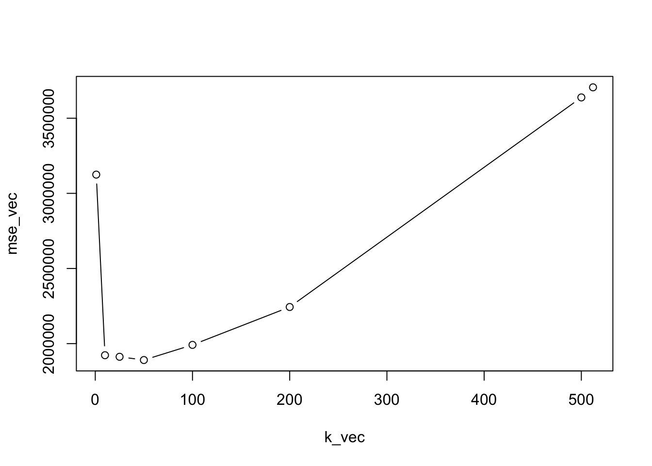
We can add some interactivity to our plot in order to better understand what’s going on:
df <- data.frame(k_vec, mse_vec)
plot_ly(df,
        x=~k_vec,
        y=~mse_vec,
        type="scatter",
        mode="lines+markers",
        text = ~paste("Considered neighbours: ", k_vec, '<br>Validation MSE:', round(mse_vec)),
        name="myfirstvec") %>%
  layout(xaxis=list(title="K neighbours"), yaxis=list(title="Validation MSE"))
Note the U-shape of the plotted line which is typical of the test error.
The value of \(k\) which minimizes the MSE is in position 4 and is given by \(k\) equal to 50:
# Smallest MSE
MSE_KNN = min(mse_vec)
MSE_KNN
## [1] 1890743# Its position
which.min(mse_vec)## [1] 4# Corresponding value of k
k_vec[which.min(mse_vec)]## [1] 502.1.4 Assessment of the tuned model
Now we can finally calculate the Test MSE with the selected parameter
k_final <- k_vec[which.min(mse_vec)]

bike_training <- rbind(bike_validation, bike_training) # recall to rejoin together test + validation
knn_final <- knn.reg(train = dplyr::select(bike_training, atemp, hum, windspeed),
                test = dplyr::select(bike_test, atemp, hum, windspeed),
                y = bike_training$cnt,
                k=k_final)

MSE_KNN_final <- mean((bike_test$cnt - knn_final$pred)^2)
MSE_KNN_final # final MSE value
## [1] 17250302.1.5 Comparison of KNN with the multiple linear model
We consider for the same set of data also the multiple linear model with 3 regressors: \[ Y = \beta_0+\beta_1 X_1+\beta_2 X_2+\beta_3 X_3 +\epsilon \]
This can be implemented by using the lm function applied to the training set of data:
lm_bike = lm(cnt ~ atemp+windspeed+hum, data=bike_training)
summary(lm_bike)
##
## Call:
## lm(formula = cnt ~ atemp + windspeed + hum, data = bike_training)
##
## Residuals:
## Min 1Q Median 3Q Max
## -4928.3 -1036.5 -86.7 1116.6 3554.3
##
## Coefficients:
## Estimate Std. Error t value Pr(>|t|)
## (Intercept) 3858.7 367.3 10.505 < 2e-16 ***
## atemp 7552.0 360.2 20.968 < 2e-16 ***
## windspeed -4658.7 763.7 -6.100 1.87e-09 ***
## hum -3268.4 410.8 -7.957 8.50e-15 ***
## ---
## Signif. codes: 0 '***' 0.001 '**' 0.01 '*' 0.05 '.' 0.1 ' ' 1
##
## Residual standard error: 1418 on 617 degrees of freedom
## Multiple R-squared: 0.4646, Adjusted R-squared: 0.462
## F-statistic: 178.5 on 3 and 617 DF, p-value: < 2.2e-16The corresponding predictions and test MSE can be obtained as follows by making use of the predict function:
predlm = predict(lm_bike,newdata = bike_test)
MSE_lm = mean((bike_test$cnt-predlm)^2)
MSE_lm
## [1] 2090156Note that the test MSE of the linear regression model is higher than the KNN MSE with \(k=50\).
2.1.6 Comparison of KNN with the multiple linear model with quadratic terms
As a sort of “tuning”, we try to extend the previous linear model by including quadratic terms of the regressors: \[ Y = \beta_0+\beta_1 X_1+\beta_2 X_2+\beta_3 X_3 + \beta_4 X_1^2 + \beta_5 X_2^2 + \beta_6 X_3^2+\epsilon \]
This is still a linear model in the parameters (not in the variables). Polynomial regression models are able to produce non-linear fitted functions.
This model can be implemented by using the poly function (with degree=2 in this case) in the formula specification. This specifies a model including \(X\) and \(X^2\).
lm_bike2 = lm(cnt ~ poly(atemp,2) +
                    poly(windspeed,2)+
                    poly(hum,2), data=bike_training)
As before we compute the test MSE:
predlm2 = predict(lm_bike2,newdata = bike_test)
MSE_lm2 = mean((bike_test$cnt-predlm2)^2)
MSE_lm2
## [1] 18643832.1.7 Final comparison
We can now compare the MSE of the best KNN model and of the 2 linear regression models:
MSE_KNN_final## [1] 1725030MSE_lm## [1] 2090156MSE_lm2## [1] 1864383Results show that the multiple linear regression model has the worst performance. The polynomial model and the KNN with \(k=50\) have a similar performance.
2.2 KNN for classification problems
For KNN classification we will use the iris dataset which is included in R (see ?iris). It contains the measurements in centimeters of the variables sepal length and width and petal length and width, respectively, for 50 flowers from each of 3 species of iris. The species are Iris setosa, versicolor, and virginica.
glimpse(iris)## Rows: 150
## Columns: 5
## $ Sepal.Length <dbl> 5.1, 4.9, 4.7, 4.6, 5.0, 5.4, 4.6, 5.0, 4.4, 4.9, 5.4, 4.…
## $ Sepal.Width <dbl> 3.5, 3.0, 3.2, 3.1, 3.6, 3.9, 3.4, 3.4, 2.9, 3.1, 3.7, 3.…
## $ Petal.Length <dbl> 1.4, 1.4, 1.3, 1.5, 1.4, 1.7, 1.4, 1.5, 1.4, 1.5, 1.5, 1.…
## $ Petal.Width <dbl> 0.2, 0.2, 0.2, 0.2, 0.2, 0.4, 0.3, 0.2, 0.2, 0.1, 0.2, 0.…
## $ Species <fct> setosa, setosa, setosa, setosa, setosa, setosa, setosa, s…summary(iris)## Sepal.Length Sepal.Width Petal.Length Petal.Width
## Min. :4.300 Min. :2.000 Min. :1.000 Min. :0.100
## 1st Qu.:5.100 1st Qu.:2.800 1st Qu.:1.600 1st Qu.:0.300
## Median :5.800 Median :3.000 Median :4.350 Median :1.300
## Mean :5.843 Mean :3.057 Mean :3.758 Mean :1.199
## 3rd Qu.:6.400 3rd Qu.:3.300 3rd Qu.:5.100 3rd Qu.:1.800
## Max. :7.900 Max. :4.400 Max. :6.900 Max. :2.500
## Species
## setosa :50
## versicolor:50
## virginica :50
##
##
## The variable Species is the response categorical variables with 3 categories.
As usual we start with visualizing the data with a plot. In this case we represent Species as a function of Sepal.Length and Sepal.Width:
iris %>%
  ggplot()+
  geom_point(aes(Sepal.Length, Sepal.Width,col=Species))+
  geom_smooth(aes(Sepal.Length, Sepal.Width,col=Species))
## `geom_smooth()` using method = 'loess' and formula 'y ~ x'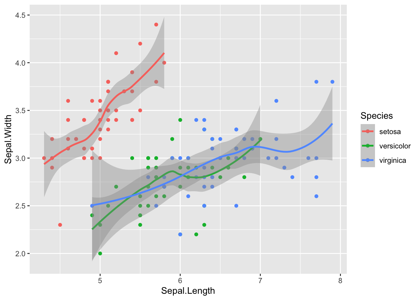 The following plot instead considers
 Species as a function of Petal.Length and Petal.Width by using separate plots:
iris %>%
  ggplot()+
  geom_point(aes(Petal.Length, Petal.Width,col=Species))+
  facet_wrap(~Species)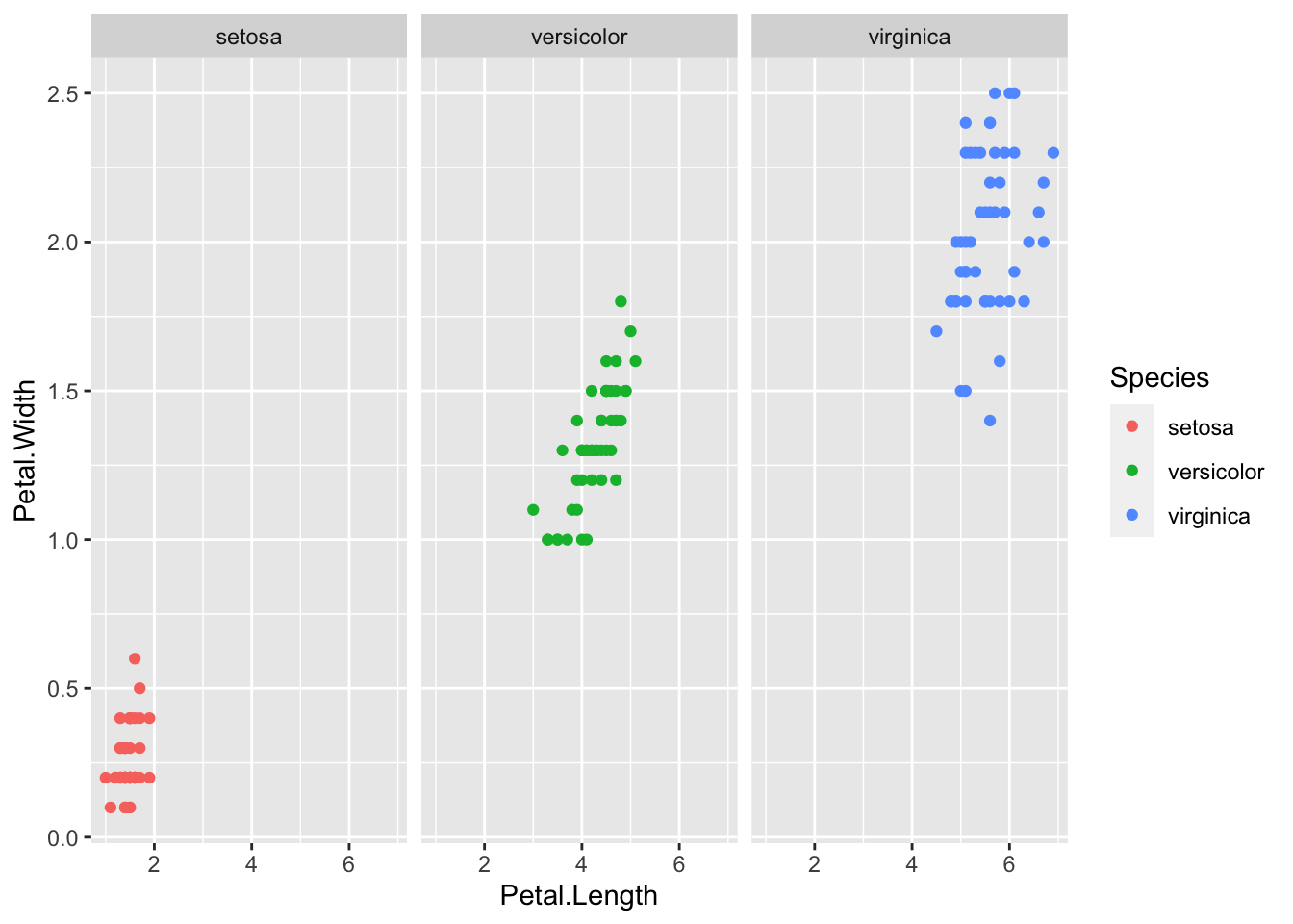
We split the dataset into 2 subsets. In other words, we are not properly tuning our algorithm, mainly because we don’t have a lot of data. More will come about it! The dataset will be:
- training set: containing 70% of the observations
- test set: containing 30% of the observations
The procedure is done randomly by using the function slice_sample. In order to have reproducible results, it is necessary to set the seed.
set.seed(1, sample.kind="Rejection")
# sample a vector of indexes/positions

iris <- iris %>% mutate(id = row_number())
iris_training <- iris %>% slice_sample(prop=0.7)
iris_test <- anti_join(x=iris, y=iris_training, by="id")
2.2.1 KNN classification with \(k=1\)
We now implement KNN classification with \(k=1\) by using the knn function from the class package (see ?knn). Note that there are two functions both named knn in the class and FNN package. In order to specify that we want to use the function in the class package we use class::knn. As before we have to specify the regressor dataframe for the training and test observations and the response variable vector (cl). The option prob makes it possible to get the probability of the majority class.
out1 = class::knn(train = dplyr::select(iris_training,-Species),
           test = dplyr::select(iris_test,-Species),
           cl = iris_training$Species,
           k = 1, #just 1 neighbors
           prob=T) # we are interest in having a look at the winning class probabilities

out1
## [1] setosa setosa setosa setosa setosa setosa
## [7] setosa setosa setosa setosa setosa setosa
## [13] setosa setosa setosa versicolor versicolor versicolor
## [19] versicolor versicolor versicolor versicolor versicolor versicolor
## [25] versicolor versicolor versicolor versicolor versicolor versicolor
## [31] versicolor versicolor virginica virginica virginica virginica
## [37] virginica virginica virginica virginica virginica virginica
## [43] virginica virginica virginica
## attr(,"prob")
## [1] 1 1 1 1 1 1 1 1 1 1 1 1 1 1 1 1 1 1 1 1 1 1 1 1 1 1 1 1 1 1 1 1 1 1 1 1 1 1
## [39] 1 1 1 1 1 1 1
## Levels: setosa versicolor virginicaPredictions are contained in the out1 object; in this case all the probabilities are equal to one because just 1 neighbor is considered (and thus the majority class will have a 100% probability).
To compare predictions \(\hat y_0\) and observed values \(y_0\) it is useful to create the confusion matrix which is a double-entry matrix with predicted and observed categories and the corresponding frequencies:
table(out1, iris_test$Species)##
## out1 setosa versicolor virginica
## setosa 15 0 0
## versicolor 0 17 0
## virginica 0 0 13In the main diagonal we can read the number of correctly classified observations. Outside from the main diagonal we have the number of missclassified observations.
The percentage test error rate is computed as follows:
#test error rate
mean(out1!=iris_test$Species)*100
## [1] 0In this case we see that 0% of the observations are missclassified.
2.2.2 KNN classification with different values of \(k\)
We now consider different values for \(k\). In particular we run the KNN algorithm for all the values of \(k\) from 1 to 100 and save the test error rate in a vector:
maxK = 100
errorrate = c()
for(i in 1:maxK){
  # KNN classification
  out = class::knn(train = dplyr::select(iris_training,-Species),
                    test = dplyr::select(iris_test,-Species),
                    cl = iris_training$Species,
                    k = i,
                    prob=T)

  # Test error rate (save in the i-th position of the vector)
  errorrate[i] = mean(out!=iris_test$Species)
}
To plot the test error rate as a function of \(k\) by using ggplot we can proceed as follows. First we need to create a new dataframe containing the values of \(k\) and of the error rate:
outfinal = data.frame(k=1:maxK,testER = errorrate)Then we plot the data
outfinal %>%
  ggplot() +
  geom_line(aes(x=k,y=testER))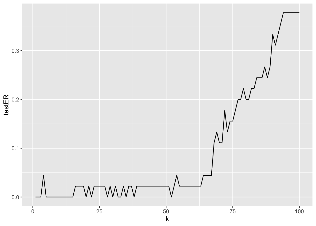
The best value of \(k\) which minimizes the test error rate is given by \(k=\) 1:
which.min(errorrate) ## [1] 1Note that there are other bigger values of \(k\) which provide the same lowest error rate (0):
which(errorrate==min(errorrate))## [1] 1 2 3 5 6 7 8 9 10 11 12 13 14 15 20 22 28 30 32 33 35 38 52This gives us the possibility to choose a different level of flexibility without worsening the test error.
2.3 Exercises Lab 1
2.3.1 Exercise 1
Use the Weekly data set contained in the ISLR package. See ?Weekly.
library(ISLR)
library(tidyverse)
?Weekly
head(Weekly)
## Year Lag1 Lag2 Lag3 Lag4 Lag5 Volume Today Direction
## 1 1990 0.816 1.572 -3.936 -0.229 -3.484 0.1549760 -0.270 Down
## 2 1990 -0.270 0.816 1.572 -3.936 -0.229 0.1485740 -2.576 Down
## 3 1990 -2.576 -0.270 0.816 1.572 -3.936 0.1598375 3.514 Up
## 4 1990 3.514 -2.576 -0.270 0.816 1.572 0.1616300 0.712 Up
## 5 1990 0.712 3.514 -2.576 -0.270 0.816 0.1537280 1.178 Up
## 6 1990 1.178 0.712 3.514 -2.576 -0.270 0.1544440 -1.372 Downglimpse(Weekly)## Rows: 1,089
## Columns: 9
## $ Year <dbl> 1990, 1990, 1990, 1990, 1990, 1990, 1990, 1990, 1990, 1990, …
## $ Lag1 <dbl> 0.816, -0.270, -2.576, 3.514, 0.712, 1.178, -1.372, 0.807, 0…
## $ Lag2 <dbl> 1.572, 0.816, -0.270, -2.576, 3.514, 0.712, 1.178, -1.372, 0…
## $ Lag3 <dbl> -3.936, 1.572, 0.816, -0.270, -2.576, 3.514, 0.712, 1.178, -…
## $ Lag4 <dbl> -0.229, -3.936, 1.572, 0.816, -0.270, -2.576, 3.514, 0.712, …
## $ Lag5 <dbl> -3.484, -0.229, -3.936, 1.572, 0.816, -0.270, -2.576, 3.514,…
## $ Volume <dbl> 0.1549760, 0.1485740, 0.1598375, 0.1616300, 0.1537280, 0.154…
## $ Today <dbl> -0.270, -2.576, 3.514, 0.712, 1.178, -1.372, 0.807, 0.041, 1…
## $ Direction <fct> Down, Down, Up, Up, Up, Down, Up, Up, Up, Down, Down, Up, Up…- How many data are available for each year? What is the temporal frequency of the data?
- Produce the boxplot which represents
Todayreturns as a function ofYear. Do you observe any difference across years? - Provide the scatterplot matrix for
TodayandLag1. Do you observe strong correlations? - Plot the distribution of the variable
Direction(with a barplot) for year 2010. Use percentage and not absolute frequencies. - Plot the distribution of the variable
Direction(with a barplot) separately for all the available years. Use percentage and not absolute frequencies. Attention: percentages should be computed by considering the number of observations available for each year and not the total number of observations. - Consider as training set the data available from 1990 to 2008 with
Lag1,Lag2andLag3as predictors andDirectionas response variable. How many data do you have in the training and test datasets? - Compute the test error rate for the KNN classifier with \(k=1\).
- Compute the test error rate for the KNN classifier for \(k\) from 1 to 50. Use the
forloop and save the results in a vector. - Plot the error rate as a function of \(k\). Which value of \(k\) do you suggest to use?
2.3.2 Exercise 2
In this exercise we will develop a classifier to predict if a given car gets high or low gas mileage using the Auto dataset. The data are included in the ISLR package (see Auto).
library(ISLR)
?Auto- Explore the data.
- Create a binary variable, named
mpg01, that is equal to 1 ifmpgis bigger than its median, and a 0 otherwise. Add the variablempg01to the existing dataframe. How many observations are classified with 1? - Study how
cylinders,weight,displacementandhorsepowervary according to the factormpg01. - Consider as training set the cars released in even years. Use as regressor the following variables:
cylinders,weight,displacementandhorsepower. How many data do you have in the training and test datasets? Suggestion: use the modulus operator%%to check if a year is even (e.g.4%%2and5%%2). - Run KNN with \(k=1\). Which is the value of the test error rate?
- Perform KNN with \(k\) from 1 to 50 using a
forloop. - Plot the test error rate as a function of \(k\).
- For which value of \(k\) do we get the lowest test error rate?
2.3.3 Exercise 3
Consider the Carseats data set available from the ISLR library. Read the help to understand which variables are available (and if they are qualitative or quantitative).
library(ISLR)
library(tidyverse)
?Carseats
Plot
Salesas a function ofPrice.Split the dataset in two separate sets: the training set with 70% of the observations and 30% for the test set. Use 14 as seed.
Fit a regression model to predict
SalesusingPrice.Compute the MSE for the model with
Salesas dependent variable andPriceas regressor.Now implement KNN regression using the same variables you used for the linear regression model above. Consider all the values of \(k\) between 1 and 200. Which is the best value of \(k\) in terms of validation error?
Compare the regression model and the KNN regression (with the chosen value of \(k\)). Which is the best model?
2.3.4 Exercise 4
This exercise uses simulated data.
Use the
rnormfunction to create a vector namedxcontaining \(n=100\) values simulated from a N(0,1) distribution. Set the seed equal to 1. These values represent the predictor’s values.Use the
rnormfunction to create a vector namedepscontaining \(n=100\) values simulated from a N(0,0.025) distribution (variance=0.025). Set the seed equal to 2. These values represent the error’s values (\(\epsilon\)).Using
xandeps, obtain a vectory(the response values) according to the following (true) model. Create also a data frame containing the values ofxandy. \[ Y = -1+0.5X+\epsilon \]Which is the length of
y? What are the values of \(\beta_0\) and \(\beta_1\) in this model?Plot the simulated data.
Fit a least squares linear model to predict
yusingx. Compare the true values of the parameters with the corresponding estimates.Display the least squares line in the scatterplot obtained before. Add to the plot also the straight line corresponding to the true model (suggestion: use
geom_abline).
Fit a polynomial regression model to predict
yusingxandx^2. Is there evidence that the quadratic term improves the model fit?Repeat points 1.-3. changing the data generation process in such a way that there is less noise in the data (the values of
xdon’t change). Consider for example a variance for the error equal to 0.001 (use a new name for the response data frame, for exampledata2). Describe your results.Repeat points 1.-3. changing the data generation process in such a way that there is more noise in the data (the values of
xdon’t change). Consider for example a variance for the error equal to 1 (use a new name for the response data, for exampledata3). Describe your results.