Practice 13 Conducting t-tests for Matched or Paired Samples in R

13.1 Directions

---

In this practice exercise, you will conduct t-test for matched or paired samples in R.

13.2 A closer look at the code

---

13.2.1 One-sample Proportion test

A study was conducted to investigate the effectiveness of hypnotism in reducing pain. Results for randomly selected subjects are shown in Table 10.11. A lower score indicates less pain. The “before” value is matched to an “after” value and the differences are calculated. The differences have a normal distribution. Are the sensory measurements, on average, lower after hypnotism? Test at a 5% significance level.

Subject:	A	B	C	D	E	F	G	H
Before	6.6	6.5	9.0	10.3	11.3	8.1	6.3	11.6
After	6.8	2.4	7.4	8.5	8.1	6.1	3.4	2.0

See EXAMPLE 10.11

13.2.1.1 What do we know?

The following is given in the question:

1. The null hypothesis is \(\overline{Pain}_{\rm after} = \overline{Pain}_{\rm before}\)
2. The alternative hypothesis is \(\overline{Pain}_{\rm after} < \overline{Pain}_{\rm before}\)

Let’s put this into r:

before <- c(6.6, 6.5, 9.0, 10.3, 11.3, 8.1, 6.3, 11.6)
after <- c(6.8, 2.4, 7.4, 8.5, 8.1, 6.1, 3.4, 2.0)

13.2.1.2 Conduct the test

To conduct a test, we need the to use the t.test() with paired = TRUE.

t.test(x=after, y=before, paired = T, conf.level = 0.95, alternative = "less")

## 
##  Paired t-test
## 
## data:  after and before
## t = -3.0359, df = 7, p-value = 0.009478
## alternative hypothesis: true difference in means is less than 0
## 95 percent confidence interval:
##       -Inf -1.174823
## sample estimates:
## mean of the differences 
##                  -3.125

With a p-value of \(0.009478\), we reject the null hypothesis.

BONUS if alternative = "two.sided" then the 95 percent confidence interval: returned by t.test() is the confidence interval for the sample proportion.

13.2.2 Repeat the same problem with a stacked data frame

Here we will create a stacked data frame out of our data. You do not need to understand how to do this for this class, but you may need to work with data in this form. So here you go.

# Create a data frame - Don't worry about this code yet
my_data <- data.frame( 
                group = rep(c("before", "after"), each = length(before)),
                weight = c(before,  after)
                )
print(my_data)

##     group weight
## 1  before    6.6
## 2  before    6.5
## 3  before    9.0
## 4  before   10.3
## 5  before   11.3
## 6  before    8.1
## 7  before    6.3
## 8  before   11.6
## 9   after    6.8
## 10  after    2.4
## 11  after    7.4
## 12  after    8.5
## 13  after    8.1
## 14  after    6.1
## 15  after    3.4
## 16  after    2.0

13.2.2.1 Conduct the test

Since we have the data organized into a stacked data frame. Making a boxplot is easy.

boxplot(my_data$weight~my_data$group)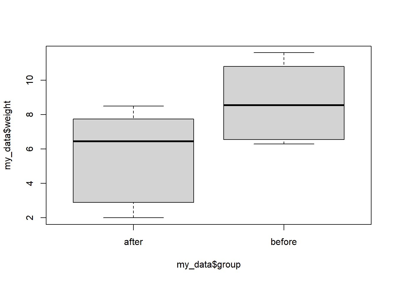

t.test(weight ~ group, data = my_data, paired = T, conf.level = 0.95, alternative = "less")

## 
##  Paired t-test
## 
## data:  weight by group
## t = -3.0359, df = 7, p-value = 0.009478
## alternative hypothesis: true difference in means is less than 0
## 95 percent confidence interval:
##       -Inf -1.174823
## sample estimates:
## mean of the differences 
##                  -3.125

We get the same conclusion as before.

13.3 Now you try

---

Use R to complete the following activities (this is just for practice you do not need to turn anything in).

A study was conducted to investigate how effective a new diet was in lowering cholesterol. Results for the randomly selected subjects are shown in the table. The differences have a normal distribution. Are the subjects’ cholesterol levels lower on average after the diet? Test at the 5% level.

Subject	A	B	C	D	E	F	G	H	I
Before	209	210	205	198	216	217	238	240	222
After	199	207	189	209	217	202	211	223	201