Practice 3 Line Plots with R
3.1 Directions
In this practice exercise, you will load data into R, and create a line plot.
3.2 A closer look at the code
Before we begin, do not worry about the first bit of code (see below). All it does is create some fake data and store it into a data frame so that we can plot it.
# Loads the tidyverse package
library(tidyverse)

data <- data.frame(year=c(1960:2019),
values1 = runif(60, -1, 1) * 10 + 1:60,
values2 = runif(60, -1, 1) * 5 + (1:60) * 0.5,
values3 = runif(60, -1, 1) * 7 + 30 - (1:60)/3)
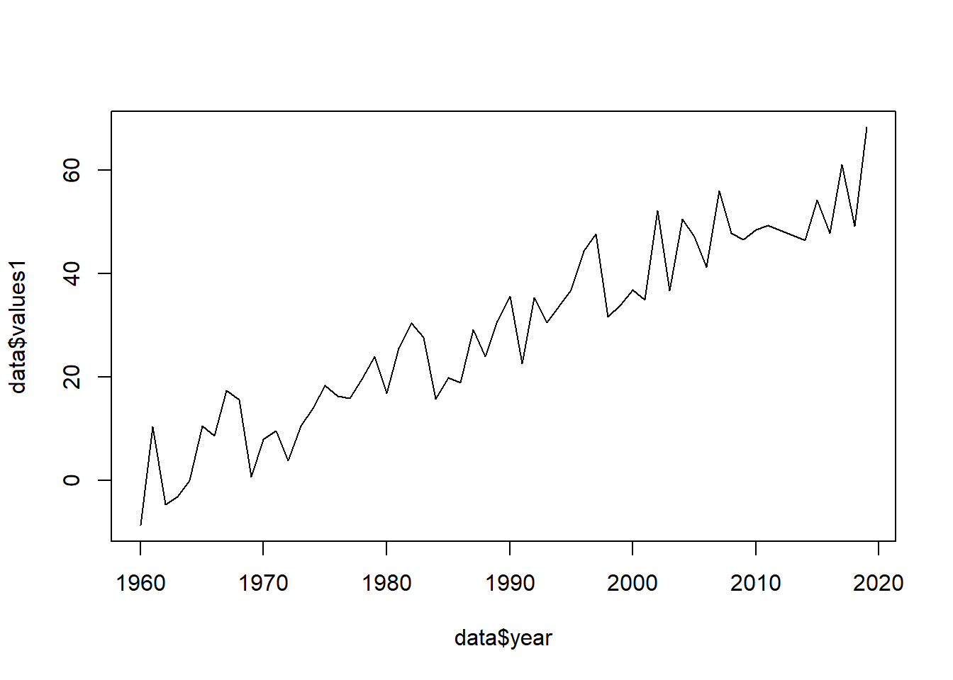
The plot command creates plots in R.
plot(x = data$year, y = data$values1, type='l')
We pass the plot command 3 arguments, or information the command needs to function.
xis the variable to be measured on the x-axis, i.e. the horizontal axisyis the variable to be measured on the y-axis, i.e. the vertical axis.type='l'indicates to R to draw a line plot.
ggplot is a very powerful data visualization package, but we will not cover ggplot until later.
3.3 R code used in the VoiceThread
# Loads the tidyverse package
library(tidyverse)

# Creates some fake data to plot
data <- data.frame(year=c(1960:2019),
values1 = runif(60, -1, 1) * 10 + 1:60,
values2 = runif(60, -1, 1) * 5 + (1:60) * 0.5,
values3 = runif(60, -1, 1) * 7 + 30 - (1:60)/3)

# Line plot in base R
plot(x = data$year, y = data$values1, type='l')

# Add points to plot
points(x = data$year, y = data$values1)

# Line plot in ggplot2
data %>% ggplot(aes(x = year, y = values1)) +
geom_line()

# Line plot in ggplot2 with groups
data %>% gather(key = "group", value = "values", -year) %>%
ggplot(aes(x = year, y = values, color = group)) +
geom_line(lwd = 1.5) +
geom_smooth(method = 'lm') +
scale_color_manual(values = c("tomato3","goldenrod","skyblue2"))
3.4 Now you try
Use R to complete the following activities (this is just for practice you do not need to turn anything in).
Plot values1 vs. year. Put year on the x-axis and values1 on the y-axis
Add points to the plot.
Example
# Generate some fake data
data <- data.frame(year=c(1960:2019),
    values1 = runif(60, -1, 1) * 10 + 1:60)
attach(data)

# Question 1
plot(x = year, y = values1, type='l')

# Question 2
points(x = year, y = values1)
R Code Window
eyJsYW5ndWFnZSI6InIiLCJwcmVfZXhlcmNpc2VfY29kZSI6IiMgR2VuZXJhdGUgc29tZSBmYWtlIGRhdGEgXG5kYXRhIDwtIGRhdGEuZnJhbWUoeWVhcj1jKDE5NjA6MjAxOSksXG4gICAgdmFsdWVzMSA9IHJ1bmlmKDYwLCAtMSwgMSkgKiAxMCArIDE6NjApXG5hdHRhY2goZGF0YSkiLCJzYW1wbGUiOiIjIFRoZSBkYXRhIGhhcyBhbHJlYWR5IGJlZW4gZ2VuZXJhdGVkIGFuZCBhdHRhY2hlZFxuXG5cbiMgUXVlc3Rpb24gMTogU3RvcmUgeW91ciBhbnN3ZXIgaW4gYGFgXG5cblxuIyBRdWVzdGlvbiAyOiBTdG9yZSB5b3VyIGFuc3dlciBpbiBgYmAiLCJzb2x1dGlvbiI6IiMgVGhlIGRhdGEgaGFzIGFscmVhZHkgYmVlbiBsb2FkZWQgYW5kIGF0dGFjaGVkXG5cbiMgUXVlc3Rpb24gMVxucGxvdCh4ID0geWVhciwgeSA9IHZhbHVlczEsIHR5cGU9J2wnKVxuXG4jIFF1ZXN0aW9uIDJcbnBvaW50cyh4ID0geWVhciwgeSA9IHZhbHVlczEpIn0=