Practical 1 Getting Started with RStudio, Data and Spatial Data
1.1 Part 1: Getting started in R / RStudio
The first part of this practical is covers some basic materials. It concentrates on working in R/RStudio and basic manipulations of data and objects defined in R.
Note: If you have not done so already, you should read the Getting Started chapter for details on how to access RStudio on a University PC (or install it on your computer), file management, working in RStudio etc.
The key things to remember are:
- R is a learning curve if you have never done anything like this before. It can be scary. It can be intimidating. But once you have a bit of familiarity with how things work, it is incredibly powerful.
- Generally, you will be working from practical worksheets and you will be provided with R scripts for each practical which have all the code.
- Your job is to try to understand what the code is doing and not to remember the code. Comments in your code really help in this regard.
- Comments are are preceded by a hash symbol
'#'- any text after these is ignored by R.
1.1.1 Introduction
You should open RStudio (see Chapter 1). Recall that RStudio is a graphical interface to R, the open source statistical package. We are using R because it has become the default tool for data science and data analytics - it does so much more than just statistics!!! When you open RStudio it looks like Figure 1.1:
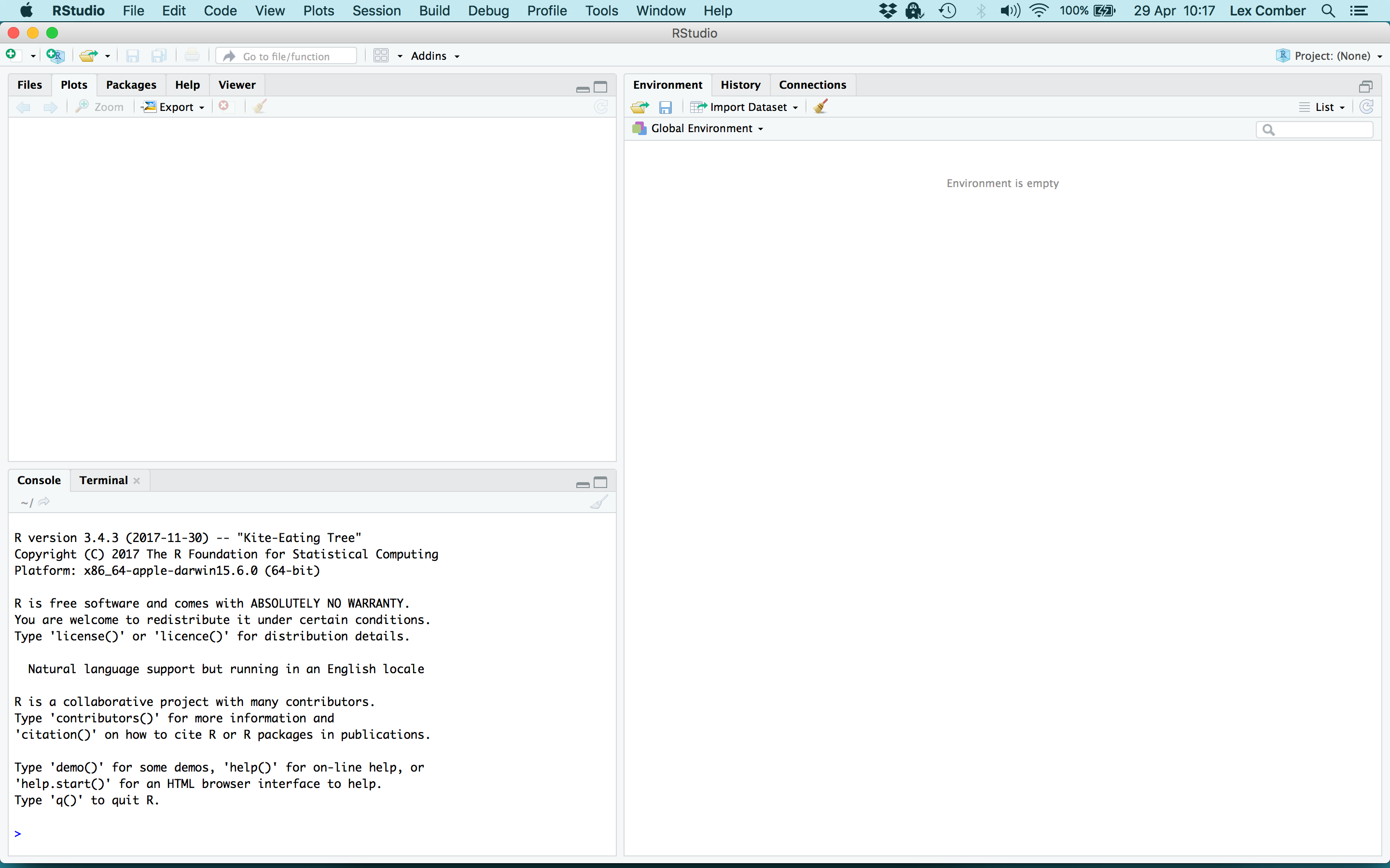
Figure 1.1: The RStudio interface.
There are a number of key points about working in RStudio :
- R code is run in the
console. - It is good practice write your code into an R
script(like a text file) in RStudio (in fact you must do this!) - As this is not a typing or English lesson, you can use the code in the scripts that are provided for you in the documents for each practical.
- You should add your comments to the script (prefaced with a hash,
#). - You should run code from the
script. - This means your code is saved, can be easily changed and re-run etc.
You should open the script for this practical practical1.R script:
File > Open File and navigate to the folder where you saved the data and files from the VLE and load the practical1.R file.
Note: The R scripts for each practical are contained in an R Scripts folder on the module VLE.
So for the first bit of R code run the code below from your R script.
To run the code (in the console pane), a quick way is to highlight the code (with the mouse or using the keyboard controls) and the press ctrl-R or cmd-Enter on a Mac. There is also a Run button at the top right of your script panel in RStudio: place your mouse cursor on the line and click on Run to run the code.
What you have done with the code snippet is assign the values to y, an R object. Assignment is the basic process of passing values to R objects.
For the purposes of this module, assignment will be done using an = (equals sign) and with a <- (less than, dash) and you can assume that = and <- are the same.
Now you can undertake operations on the objects. Write and then run the following code:
## [1] 8.6 14.2 12.6 10.4 6.4 4.2## [1] 28.2## [1] 4.7Operations undertake operations on R objects either directly, using mathematical notation like * for multiply or functions like max to find the maximum value in an R object.
Note: You should note that functions are always followed by round brackets (). These are different from square and curly brackets ([ ]) and curly ones { \}. Functions always return something and have the form:
You can examine the arguments or parameters that a function takes by examining the help for it. For example
And…
Note: It is good practice to write comments in your code. Comments are prefixed by # and are ignored by R when entered into the console. Run the code below into your R script and run it. R ignores everything after the hash (#).
You should remember to write your code and add comments as these will help you understand your code and what you did when come back to it at a later date.
1.1.2 Basic data types in R
The preceding sections created a number of R objects. You should see them in the Environment pane in RStudio or listing them by entering ls() at the console. There are a number of fundamental data types in R that are the building blocks for data analysis. The sections below explore different data types and illustrate further operations on them.
1.1.2.1 Vectors
Examples of vectors are:
# numeric
c(2,3,5,2,7,1)
# The numbers 3, 4, .., 10
3:10
# logical
c(TRUE,FALSE,FALSE,FALSE,TRUE,TRUE,FALSE)
# character
c("London","Leeds","New York","Montevideo", NA)
Vectors may have different modes such as logical, numeric or character. The first two vectors above are numeric, the third is logical (i.e. a vector with elements of mode logical), and the fourth is a string vector (i.e. a vector with elements of mode character). The missing value symbol, which is NA, can be included as an element of a vector.
The c in c(2, 3, 5, 7, 1) above is an acronym for concatenate, i.e. the meaning is: Join these numbers together in to a vector. Existing vectors may be included among the elements that are to be concatenated. In the following code, we form vectors x and y (overwriting those that the x and y that were defined earlier) which we then concatenate to form a vector z:
## [1] 2 3 5 2 7 1## [1] 10 15 12## [1] 2 3 5 2 7 1 10 15 12The concatenate function c() may also be used to join lists.
Vectors can be subsetted. There are two common ways to extract subsets from vectors. Note in both cases, the use of the square brackets [ ].
- Specify or index the elements that are to be extracted, e.g.
## [1] 3 2Note that negative numbers can be used to omit specific vector elements:
## [1] 2 2 7 1- Specify a vector of logical values to select elements. The elements that are extracted are those for which the logical value is
TRUE. Thus suppose we want to extract values ofxthat are greater than 4.
## [1] 5 7Examine the logical selection:
## [1] FALSE FALSE TRUE FALSE TRUE FALSEA number of relations may be used in the extraction of subsets of vectors are < <= > >= == !=. The first four compare magnitudes, == tests for equality, and != tests for inequality.
1.1.2.2 Matrices and Data Frames
The fundamental difference between a matrix and data.frame are that matrices can only contain a single data type - numeric, logical, text etc. Whereas a data frame can have different types of data in each column, with all elements of any column being of the same type i.e. all numeric, all factors, all logical, all character, etc.
Matrices are easy to define:
##      [,1] [,2]
## [1,]    1    6
## [2,]    2    7
## [3,]    3    8
## [4,]    4    9
## [5,] 5 10## [,1] [,2]
## [1,] 1 2
## [2,] 3 4
## [3,] 5 6
## [4,] 7 8
## [5,] 9 10## [,1] [,2]
## [1,] "a" "f"
## [2,] "b" "g"
## [3,] "c" "h"
## [4,] "d" "i"
## [5,] "e" "j"Many R packages come with datasets. The iris dataset is an internal R dataset and is loaded to your R session with the code below.
This a data.frame:
## [1] "data.frame"The code below uses the head() function to print out the first 6 rows and the dim() function to tell us the dimensions of iris.
##   Sepal.Length Sepal.Width Petal.Length Petal.Width Species
## 1          5.1         3.5          1.4         0.2  setosa
## 2          4.9         3.0          1.4         0.2  setosa
## 3          4.7         3.2          1.3         0.2  setosa
## 4          4.6         3.1          1.5         0.2  setosa
## 5          5.0         3.6          1.4         0.2  setosa
## 6 5.4 3.9 1.7 0.4 setosa## [1] 150 5The str() function can be used to indicate the formats of the attributes (columns, fields) in iris:
## 'data.frame':    150 obs. of  5 variables:
##  $ Sepal.Length: num  5.1 4.9 4.7 4.6 5 5.4 4.6 5 4.4 4.9 ...
##  $ Sepal.Width : num  3.5 3 3.2 3.1 3.6 3.9 3.4 3.4 2.9 3.1 ...
##  $ Petal.Length: num  1.4 1.4 1.3 1.5 1.4 1.7 1.4 1.5 1.4 1.5 ...
##  $ Petal.Width : num  0.2 0.2 0.2 0.2 0.2 0.4 0.3 0.2 0.2 0.1 ...
##  $ Species     : Factor w/ 3 levels "setosa","versicolor",..: 1 1 1 1 1 1 1 1 1 1 ...
Here we can see that 4 of the attributes are numeric and the other is a factor (a kind of ordered categorical variable).
The summary() function is also very useful and shows different summaries of the individual attributes (columns) in iris.
##   Sepal.Length    Sepal.Width     Petal.Length    Petal.Width
##  Min.   :4.300   Min.   :2.000   Min.   :1.000   Min.   :0.100
##  1st Qu.:5.100   1st Qu.:2.800   1st Qu.:1.600   1st Qu.:0.300
##  Median :5.800   Median :3.000   Median :4.350   Median :1.300
##  Mean   :5.843   Mean   :3.057   Mean   :3.758   Mean   :1.199
##  3rd Qu.:6.400   3rd Qu.:3.300   3rd Qu.:5.100   3rd Qu.:1.800
##  Max.   :7.900   Max.   :4.400   Max.   :6.900   Max.   :2.500
##        Species
##  setosa    :50
##  versicolor:50
##  virginica :50
##
##
##
The main R graphics function is plot() and when it is applied to a data frame or it a matrix shows how attribute values correlate to each other. There are various other alternative helpful forms of graphical summary. The scatterplot shown in Figure 2 is of the first 4 fields (columns) in iris. Note how the inclusion of upper.panel=panel.smooth causes the lowess curves to be added to Figure 1.2.
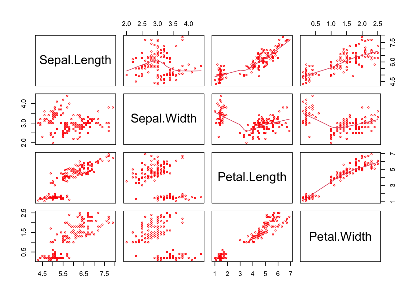
Figure 1.2: A plot of the numeric variables in the iris data.
The individual data types can also be investigated using the sapply() function. This applies a function to each column in matrix or data frame:
A key property in a data.frame is that columns can be vectors of any type. It is effectively a list (group) of column vectors, all of equal length.
Further Data types There are many more data types in R. Chapter 1 in Comber and Brunsdon (2021) provides a brief introduction to some of the important ones, and Chapter 2 in [Brunsdon and Comber (2018) provides a comprehensive overview with worked examples and exercises.
1.1.3 Basic data selection operations - indexing
In the examples above you undertook some selection from vectors to create subsets. This is known as indexing. For example, in the plot call above there are number of things to note (as well as the figure). In particular note the use of the vector 1:4 to index the columns of iris:
Notice that 1:4 extracted all the columns between 1 and 4 - very useful.
This hints at how elements of flat data tables such as matrices and data frames can be extracted and / or ordered by using square brackets. Run the code below.
Notice a number of things:
- In the second line of the code above, the 1st and 4th elements from the vector of column names were selected.
- In the third line the 4th and 1st elements were extracted in that order!
- For the plot, a vector was passed to the second argument, after the comma, in the square brackets
[,]to indicate which columns were to be plotted.
Indexing in this way is very important: the individual rows and columns of 2 dimensional data structures like data frames, matrices, tibbles etc can be accessed by passing references to them in the square brackets.
Such indexing could of course have been assigned to an R object and then used to do the subsetting.
This is a Key Point: Data held in data tables (and arrays) in R can be accessed using some simple square brackets notation as follows: dataset[rows, columns]]:
Specific rows and columns can be selected using a pointer or an index. An index tells R which rows and / or columns to select and can be specified in 3 main ways :
- numerically - the code below returns the first 10 rows and 2 columns
- by name - the code below returns the first 10 rows and 2 named columns
- logically - the code below returns the first 10 rows and 2 logically selected columns
Thus there are multiple ways in which the \(n^{th}\) rows or columns in a data table can be accessed.
Also note that compound logical statements can be used to create an index:
Different binary operators for generating logical statements can be found at:
And the syntax for compound logical statements - you will principally be interested in and (&) and or (|)
1.2 Part 2: Data and Spatial Data
1.2.1 Introduction: packages and data files
The base installation of R includes many functions and commands. However, more often we are interested in using some particular functionality, encoded into packages contributed by the R developer community. Installing packages for the first time can be done at the command line in the R console using the install.packages command as in the example below to install the tidyverse library or via the RStudio menu via Tools > Install Packages.
When you install packages you should also install their dependencies - other packages that are required by the package that is being installed. This can be done by selecting check the box in the menu or including dep = TRUE as in the commands below.
Run the code below this may take some time. The first code block below tests for the presence of the packages and if they are not present, installs them:
packages <- c("sf", "tidyverse", "cols4all")
# check which packages are not installed
not_installed <- packages[!packages %in% installed.packages()[, "Package"]]
# install missing packages
if (length(not_installed) > 0) {
  install.packages(not_installed, repos = "https://cran.rstudio.com/", dep = T)
}
When this is done, these packages can be loaded into your current R session using the library function:
# load the packages
library(sf)         # for spatial data
library(tidyverse)  # for data wrangling
library(cols4all)   # for graphics
There are a number of ways of loading data into your R session:
- read a local file in proprietary format (e.g. an Excel file or
.csvfile). - read a local R formatted binary file (typically with an
.rdaor.RDataextension). - download and manipulate data from the internet.
- read a file from somewhere in the internet (proprietary or R binary format).
Before any reading and writing you should make sure that your R session is pointing at your working directory for this Session. This is so the data that you downloaded and moved to a folder can be fund and read in by T. This can be done in a number of ways. One way is to use the menu system:
Session > Set Working Directory … which give you options to chose from. If you have an R script in the correct directory (e.g. prac1.R) with your data, then you can chose > To Source File Location.
This will initiate a setwd() call in your console that you can copy over to your script.
Another way is to use the setwd() function directly, but you have to know the full path to your folder (you should be using the M drive for this module!):
1.2.1.1 Loading and saving data in.txt and .csv format
The base installation of R comes with core functions for reading and writing .txt, csv and other tabular formats to save and load data to and from local files.
To read (load) a spreadsheet file make sure you have set the working directory to the folder containing the liverpool_oa.csv file, as above.
Note: All the data files for this module are contained a Data folder on the module VLE.
Next, read the file into RT. The code below reads it into an R object called oa and the use of header=TRUE causes R to use the first line to get header information for the columns.
The oa data object in your R environment represents census Output Areas (~300 people) in Liverpool and contains census data of economic well-being (unemployment and percentages - unmplyd), life-stage indicators (percentage of under 16 years (u16), 16-24 years (u25), 25-44 years (u45), 45-64 years (u65) and over 65 years (o65) and an environmental variable of the percentage of the census area containing greenspaces. The unemployment and age data were from the 2011 UK population census (https://www.nomisweb.co.uk) and the greenspace proportions were extracted from the Ordnance Survey Open Greenspace layer (https://www.ordnancesurvey.co.uk/opendatadownload/products.html). It also contains the coordinates of the geometric centre of the census area in OSGB projection.
Examine the contents of oa:
The object oa is a data.frame.
Data frames are ‘flat’ in that they typically have a rectangular layout like a spreadsheet, with rows typically relating to observations (individuals, areas, people, houses, etc) and columns their properties or attributes (height, age, etc). The columns in data frames can be of different types: vectors of numbers, factors (classes) or text strings. Data frames are central to the way that all of the more recent R routines process data. For now, think of data frames as like spreadsheets, where the rows are observations and the columns are fields or variables.
Notice that oa object includes the OAC_class (the Output Area geodemographics classification - see Vickers and Rees (2007) and Gale et al. (2016)).
You can save a copy of this data table to your local folder.
You should check that the file has been created in your working directory and you may want to open it with Excel or similar.
A further data table format is the tibble, defined in dplyr as part of the the tidyverse package.
The tibble is a reworking of the data.frame. It is a definite upgrade. It retains the advantages of the data.frame formats (multiple data types, for example) and eliminates less effective aspects related to partial matching. The print method for tibble returns the first 10 records by default, whereas for data.frame all records are returned. The tibble class also includes a description of the class of each field (column) when it is printed.
The code below converts the oa data.frame to a tibble. You should note the differences between these data table formats:
## # A tibble: 1,584 × 11
##    code      gs_area   u16   u25   u45   u65   o65 unmplyd OAC_class     Easting
##    <chr>       <dbl> <dbl> <dbl> <dbl> <dbl> <dbl>   <dbl> <chr>           <dbl>
##  1 E00032991   2.28   5.62 20.9   45.9 26.2   1.25   18.1  Ethnicity Ce… 335715.
##  2 E00032992   0      7.5  21.7   48.3 18.3   4.17   25.2  Ethnicity Ce… 335882.
##  3 E00032993   0      9.93 25.9   46.8  9.93  7.45   10.3  Ethnicity Ce… 335406.
##  4 E00033032   4.01   3.75 14.4   56.5 17.6   7.78    9.73 Cosmopolitans 336792.
##  5 E00033034   3.26   5.11 12.8   64.5 14.4   3.19    6.72 Cosmopolitans 337013.
##  6 E00033035   0      9.47  8.08  38.7 23.7  20.1    10.1  Constrained … 337243.
##  7 E00033036   0      8.38  5.76  54.5 26.2   5.24   10.6  Ethnicity Ce… 337300.
##  8 E00033037   0      9.24  3.50  27.1 22.6  37.6     4.35 Urbanites     338980.
##  9 E00033038   0.207  9.04 10.8   57.2 21.1   1.81    6.25 Cosmopolitans 337270.
## 10 E00033040   0     13.7  13.7   39.3 20    13.3    10.1  Ethnicity Ce… 337413.
## # ℹ 1,574 more rows
## # ℹ 1 more variable: Northing <dbl>
If you finish early or later when you return to this practical in your own time, you should examine the tibble vignette and explore the sections on creation, coercion, subsetting etc:
Data Tasks
You will need to write some code that does the following:
- Selects the 9th, 99th and 999th records from
oa - Selects the records from
oawith more than 25% green space in area - Selects the
codeandOAC_classfields (columns) fromoa - Selects every 9th record from
oa(hint useseq) - Extracts the numeric variables from
oaand assigns them to new objectoa2:
The answers to the tasks are at the end of the worksheet.
1.2.2 Spatial Data
This section covers the following topics:
- spatial data formats:
spvssfformats - reading and writing spatial data
- some initial mapping of spatial data
The spatial frameworks in this part of the practical were from the EDINA data library (https://borders.ukdataservice.ac.uk). The OAs and LSOAs are both projected to the OSGB projection (EPSG 27700). The OA layer also has a geo-demographic class label (OAC_class) from the OAC (see Gale et al. (2016)) of 8 classes.
1.2.2.1 Spatial data formats: sf vs sp
For many years the tools for handling spatial data in R were built around the spatial data structures defined in the sp package. The sp class of objects are broadly analogous to shapefile formats (lines points, areas) and raster or grid formats. The sp format defined spatial objects with a data.frame (holding attributes) and without (purely spatial objects).
However, recently a new class of spatial object has been defined called sf or Simple Feature. An overview of the evolution of spatial data in R can be found at https://edzer.github.io/UseR2017/. The sf format seeks to encode spatial data in a way that conforms to a formal standard (ISO 19125-1:2004). This emphasises the spatial geometry of objects, their hierarchical ordering and the way that objects are stored in databases. The aim of the team developing sf (actually many of them are the same people who developed sp so they do know what they are doing!!) is to provide a new consistent and standard format for spatial data in R.
In this module, all spatial data will mainly be held and analysed in sf format. However, many functions for spatial analysis still only work with sp format objects and there are functions to transform spatial data between these formats.
1.2.2.2 Reading and writing spatial data
The code below creates a point spatial dataset in sf format from the oa data table using the coordinates and information about the geographical projection:
Here the coordinate reference system is 27700. This is the OSGB projection - see https://epsg.io/27700
And you can examine what was created:
Notice, that like tibble format data tables, just the first 10 records are printed out by default rather than all of them.
The st_read function can be used to read data into the R session:
We can examine spatial data in the same way as non-spatial data:
1.2.2.3 Mapping spatial data
These data attributes can be mapped using the code below as in the map below using the geom_sf() function from the ggplot2 package loaded as part of the tidyverse package as in Figure \(\ref{fig:ch1fig3}\):
# call ggplot
ggplot() +
  # specify that geometry is being plotted
  geom_sf(data = oa_sf2, aes(fill = gs_area), colour = NA) +
  # change the default shading
  scale_fill_continuous(type = "viridis")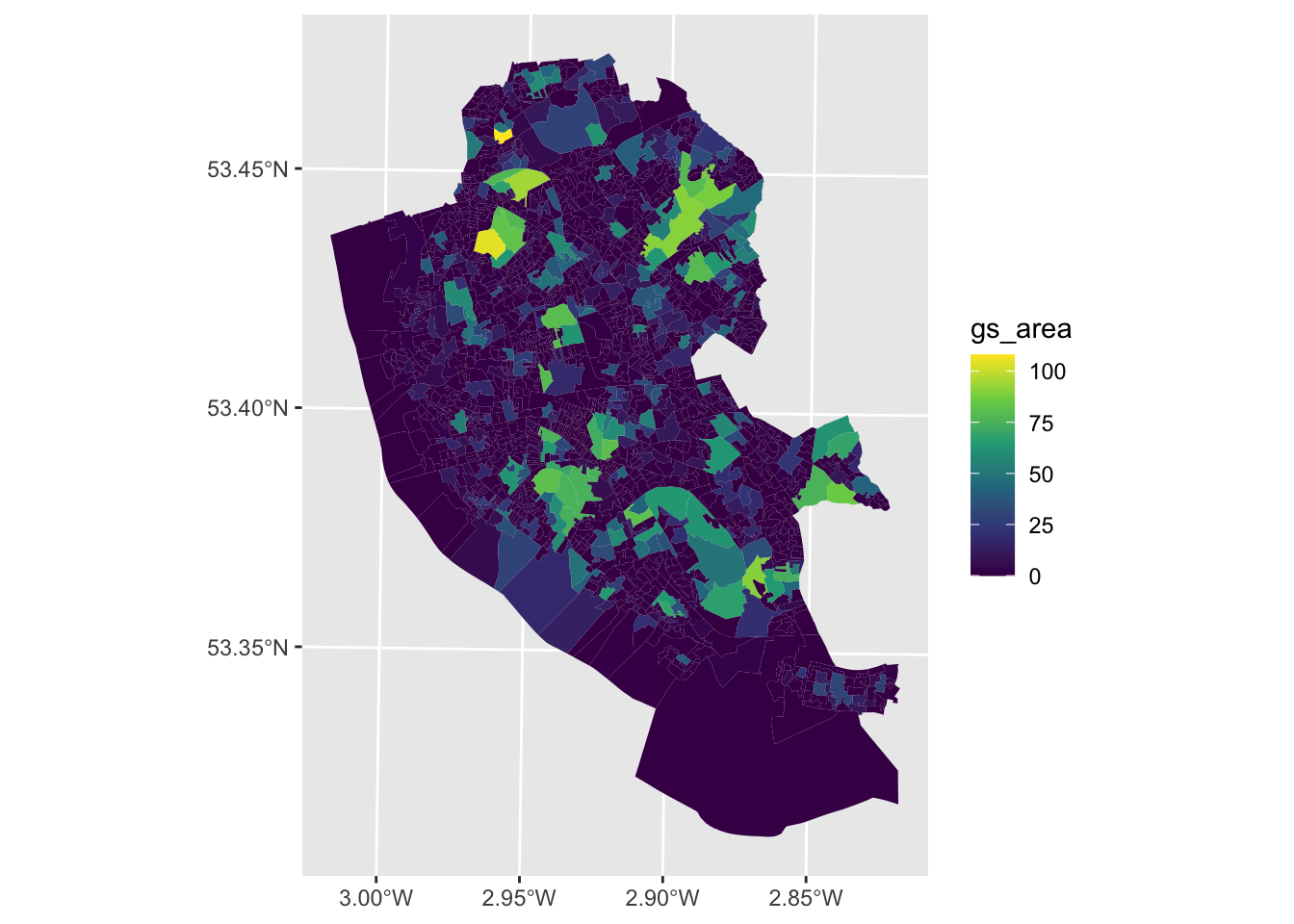
Figure 1.3: A map of Green Space % in Liverpool Ouput Areas.
We will cover graphics with ggplot in more detail later in the module.
When you return to this session after the practical you should examine the sf vignettes. These include an overview of the format, reading and writing from and to sf formats including conversions to and from sp and sf, and some illustrations of how sf objects can be manipulated. The code below will create a new window with a list of all of the sf vignettes:
A full description of the sf format can be found in the sf1 vignette:
Spatial Data Tasks
- Write some code that writes the records (areas) in
oathat have anOAC_classofEthnicity Centralto a file calledpolys.shpusing thest_writefunction (hint have a look at the help forst_write). - Write some code that maps the unemployed attribute in
oa_sf(unmplyd).
1.2.3 Some basic visualisations
The preceding sections have illustrated a number of different data structures in R, mostly in a flat data table format. Later in the module, the ggplot2 packages for visualising data (as used above in the maps) will be formally introduced. As a background to this it is important to cover some basic plot and data visualisation, using scatterplots, histograms and boxplots.
The simplest plot is a histogram of a single variable as in Figure 1.4:
hist(oa$unmplyd, xlab='Unemployment %', main='Histogram of Unemployment %',
     col = 'DarkRed', breaks = 20)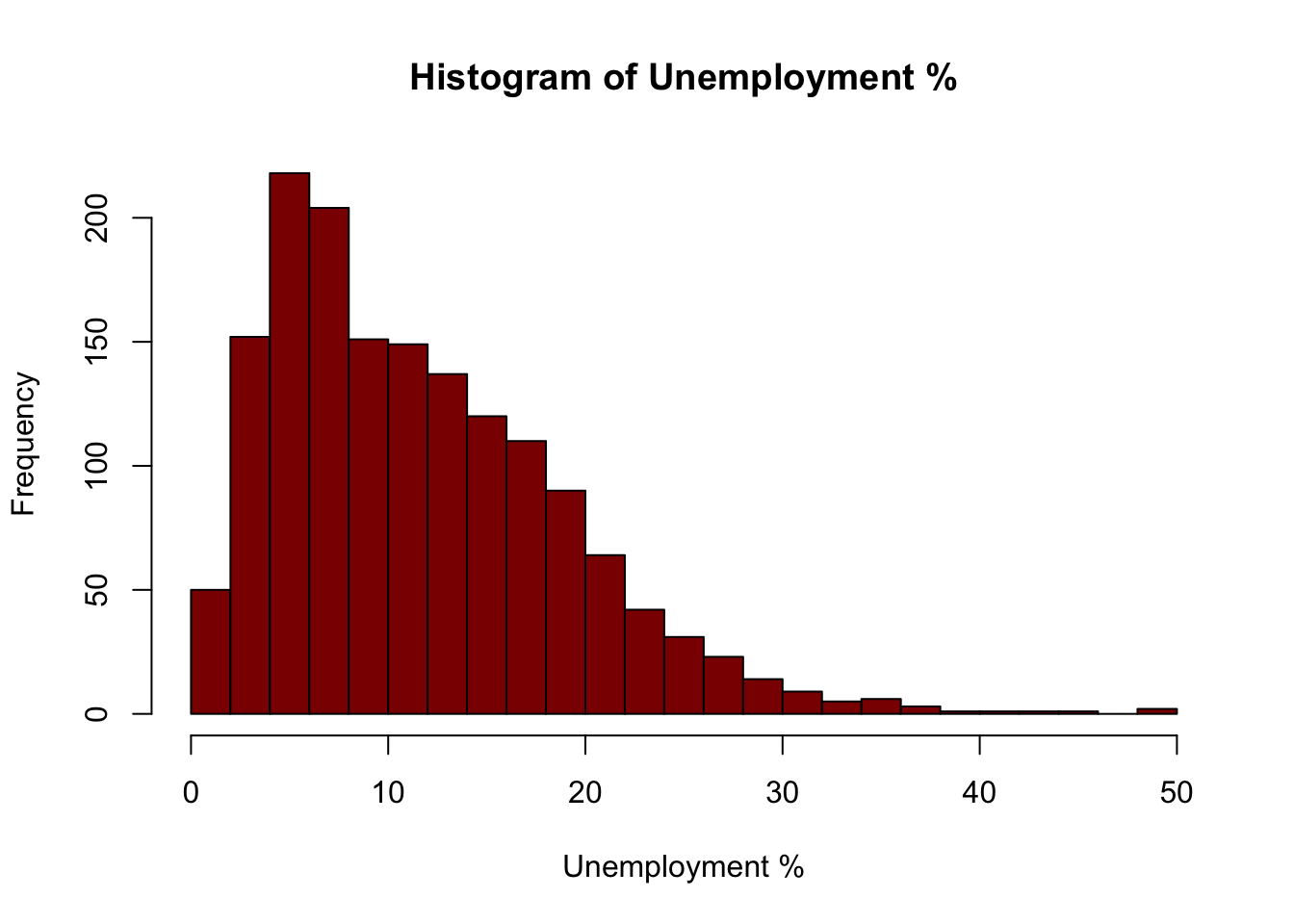
Figure 1.4: An example of a simple histogram.
A summary of a single variable is provided by a boxplot
This can be expanded to look at the distributions across groups, in this case Unemployment with OAC class as in Figure 1.5.
boxplot(oa$unmplyd~oa$OAC_class,
        # the palette
        col = c4a("brewer.spectral"),
        # the axis text size and orientation
        cex.axis = 0.7, las = 2,
        # the axis labels
        xlab = "", ylab = "Unemployed %",
        # the category names
        names = c("Constrained", "Cosmopolitans", "Eth. Central", "Hard-Pressed",
                  "Multicultural", "Suburbanites", "Urbanites"))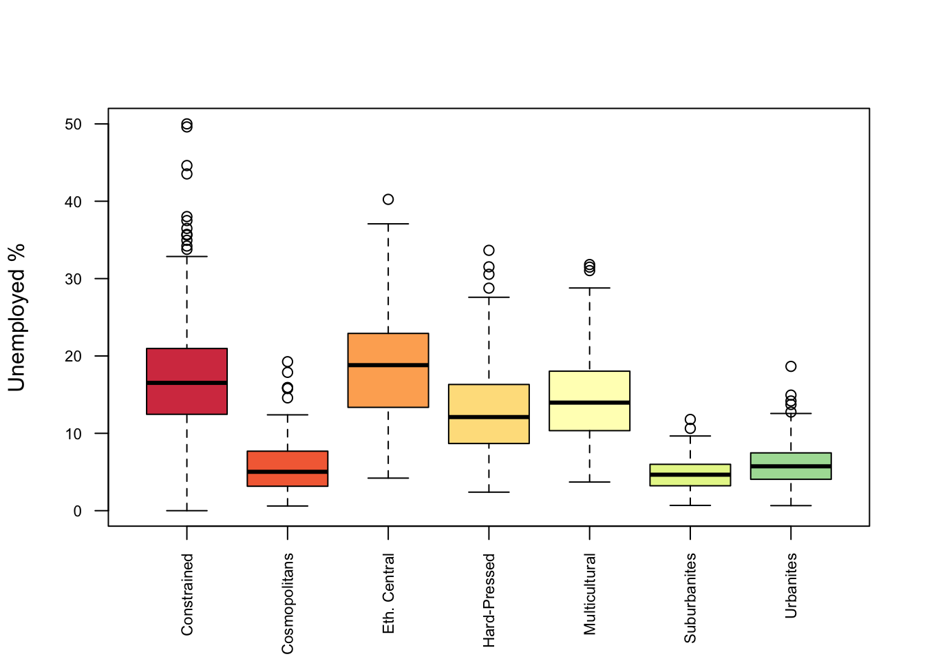
Figure 1.5: A boxplot of relationships between categorical and numeric variables.
If you want to examine the various palettes in the c4a package enter :
Or try the below but remember to escape the interface using the esc key!
The scatterplot provides the simplest way of examining how 2 numeric variables interact as has been used earlier. This allows the relationships (correlations) between continuous variables to be examined as in Figure 1.6.
plot(oa$u25, oa$o65,
     cex = 0.5,
     col ="dodgerblue",
     main ="A scatterplot with trend line")
# add a regression trend line
abline(lm(oa$o65~oa$u25), lty = 2, col = "darkblue", lwd = 2)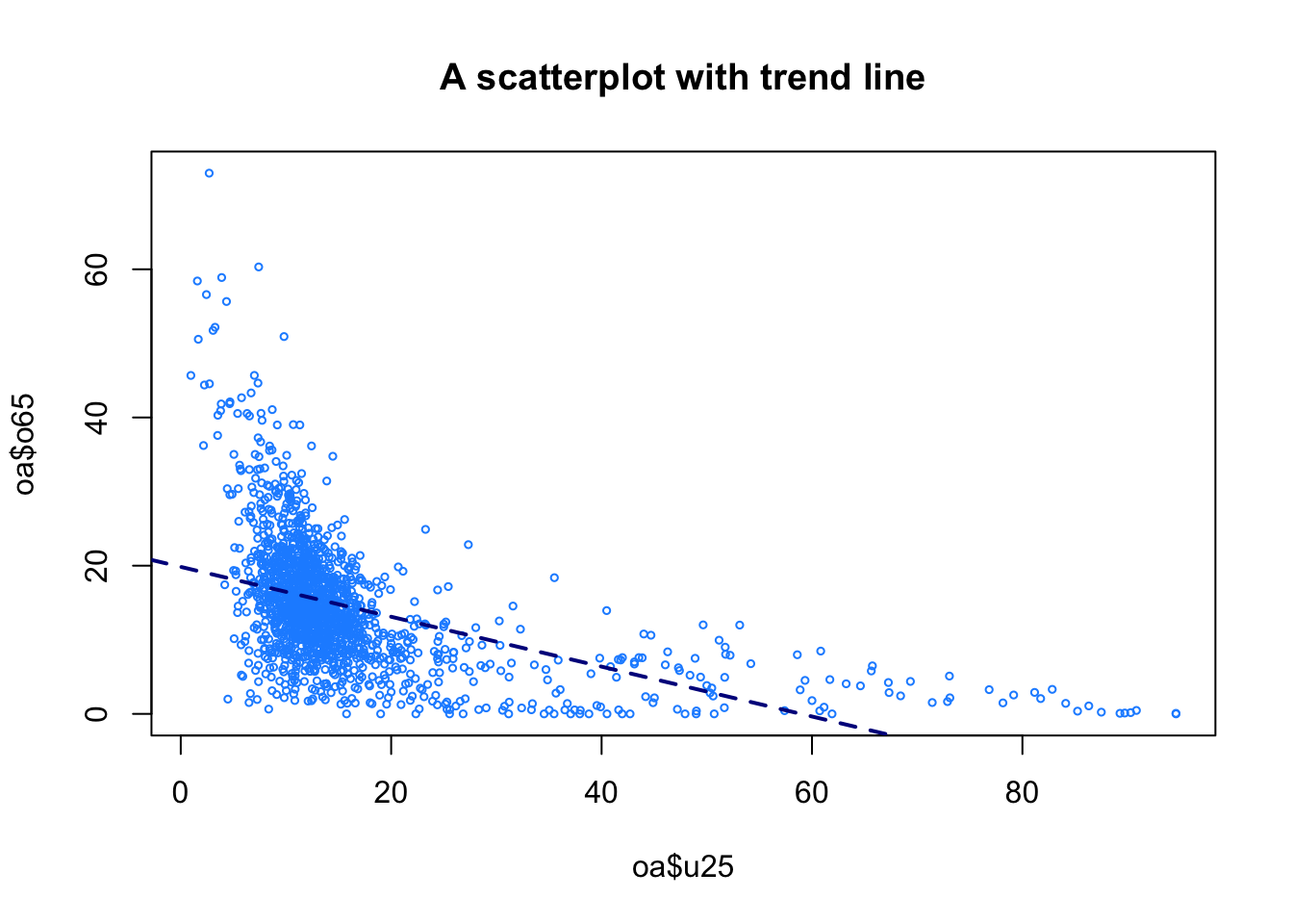
Figure 1.6: A basic plot of relationships between numeric variables.
This is only a short introduction to basic visualisations. We will develop more complex and sophisticated visual data summaries in future weeks.
1.3 Answers to Tasks
1.3.1 Data Tasks
- Select the 9th, 99th and 999th records from
oa
- Select the records from
oawith more than 25% green space in area
- Selects the
codeandOAC_classfields (columns) fromoa
- Selects every 9th record from
oa(hint useseq)
- Extracts the numeric variables from
oaand assigns them to new objectoa2:
1.3.2 Spatial Data Tasks
- Write some code that writes the records (areas) in
oathat have anOAC_classofEthnicity Centralto a file calledpolys.shpusing thest_writefunction (hint have a look at the help forst_write).
index = oa_sf$OAC_class == "Ethnicity Central"
st_write(oa_sf[index,], "polys.shp", delete_layer = T, driver = "ESRI Shapefile")- Write some code that maps the unemployed attribute in
oa_sf(unmplyd).
1.4 Useful Video Links
- a short introduction to R: https://www.youtube.com/watch?v=FY8BISK5DpM
- R programming in one hour - a crash course for beginners: https://www.youtube.com/watch?v=eR-XRSKsuR4 - this might make more sense after Practical 2