5 Time series
Install/load libraries/used data
if (!require(openxlsx)) install.packages('openxlsx')
library(openxlsx)
if (!require(patchwork)) install.packages('patchwork')
library(patchwork)
if (!require(urca)) install.packages('urca')
library(urca)
if (!require(GGally)) install.packages('GGally')
library(GGally)
if (!require(pxR)) install.packages('pxR')
library(pxR)
if (!require(fpp3)) install.packages('fpp3')
library(fpp3)
if (!require(tidyverse)) install.packages('tidyverse')
library(tidyverse)
source("utilidades.R")
Time series are data that change over time, such as the world population over the years or the daily sales data of a company or the hourly energy consumption in a city. Given their great importance, we will dedicate this chapter to studying them as a special case of exploratory data analysis. Here we will see a brief introduction to the topic. For a more detailed analysis see, for example, [HyAt21].
5.1 tsibble objects
To store and manage time series we will use a special type of object called tsibble from the fpp3 library specialized in time series management. Essentially a tsibble is a tibble in which one of the variables is a temporary variable that is managed in a special way. We are going to introduce the characteristics of a tsibble object through an example: we are going to read a table with data on the annual evolution of the population by countries and regions where we will select the world population and that of three continents.
owid_population <- read_csv("https://ctim.es/AEDV/data/owid_population.csv") %>%
   as_tibble() %>%
   filter(
     Entity == "World" |
     Entity == "Europe" |
     Entity == "Asia" |
     Entity == "Africa"
   )
owid_population
## # A tibble: 888 × 4
## Entity Code Year `Population (historical estimates)`
## <chr> <chr> <dbl> <dbl>
## 1 Africa <NA> 1800 81273172
## 2 Africa <NA> 1801 81313551
## 3 Africa <NA> 1802 81418900
## 4 Africa <NA> 1803 81525621
## 5 Africa <NA> 1804 81633731
## 6 Africa <NA> 1805 81743247
## 7 Africa <NA> 1806 81854174
## 8 Africa <NA> 1807 81966528
## 9 Africa <NA> 1808 82080332
## 10 Africa <NA> 1809 82195596
## # ℹ 878 more rowsNext we build a tsibble from this table
tsibble(
   date = owid_population$Year,
   population = owid_population$`Population (historical estimates)`,
   location = owid_population$Entity,
   index = date,
   key = location
)
One of the tsibble variables is always a temporary data, in this example, the year. When building the tsibble you must identify that variable using the name index. Furthermore, when, as in this case, there are several time series, the variable (or variables) that identify these time series must be identified with the name key in such a way that for each combination of the index and key variables there is, at most, a single row (record) in the table.
The previous portion of code to create a tsibble is equivalent to the following where we build the tsibble by adding to a tibble the information about which variables correspond to index and key:
owid_population <- owid_population %>%
   select(
     date=Year,
     population=`Population (historical estimates)`,
     location=Entity
   )%>%
   as_tsibble(index = date,key=location)
owid_population
## # A tsibble: 888 x 3 [1Y]
## # Key: location [4]
## date population location
## <dbl> <dbl> <chr>
## 1 1800 81273172 Africa
## 2 1801 81313551 Africa
## 3 1802 81418900 Africa
## 4 1803 81525621 Africa
## 5 1804 81633731 Africa
## 6 1805 81743247 Africa
## 7 1806 81854174 Africa
## 8 1807 81966528 Africa
## 9 1808 82080332 Africa
## 10 1809 82195596 Africa
## # ℹ 878 more rowsDifferent formats can be used for the temporary variable index. The following functions allow format changes for tsibble from a variable of type date.
## <yearquarter[1]>
## [1] "2022 Q3"
## # Year starts on: January## <yearmonth[1]>
## [1] "2022 jul."## <yearweek[1]>
## [1] "2022 W26"
## # Week starts on: Monday## [1] "2022-07-01"5.2 Visualization
Let’s visualize these time series using the autoplot function:
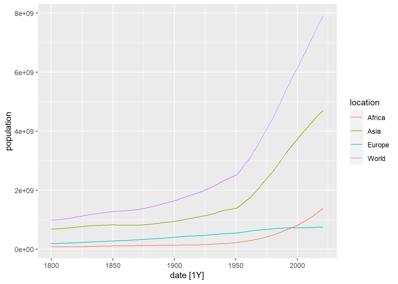
Figure 5.1: Drawing of the evolution of population in the world, Africa, Asia and Europe using autoplot
Below we draw the same series, separating each one on a graph:
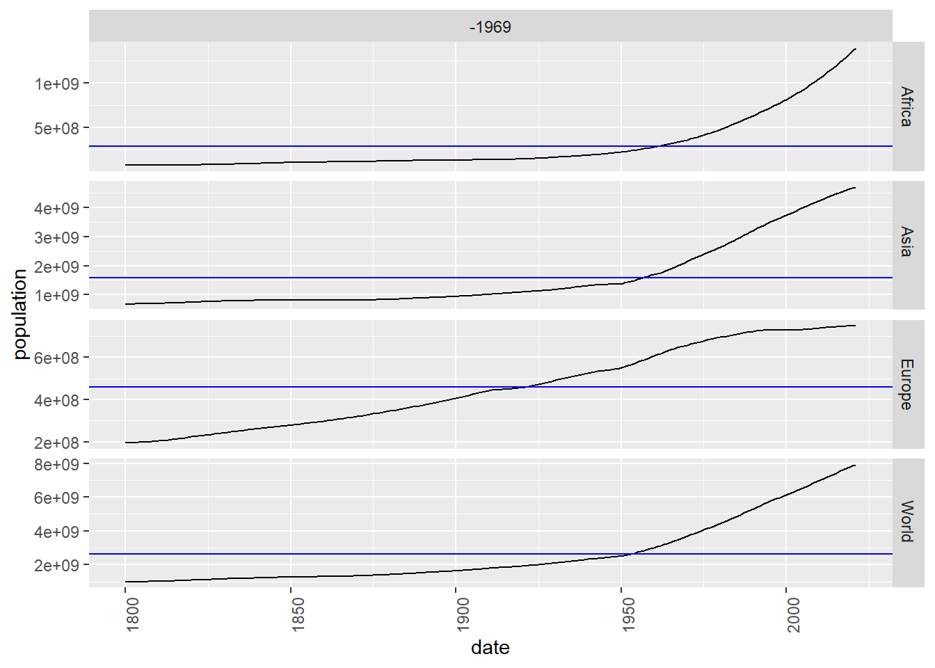
Figure 5.2: Separate drawing of the evolution of population in the world, Africa, Asia and Europe using gg_subseries
Now we do the same but putting the graphs in the form of a grid. As we can see, it is possible to use the ggplot function to draw tsibbles:
owid_population %>%
ggplot(aes(x=date,y=population)) +
geom_line() +
facet_wrap(~location,scales = "free")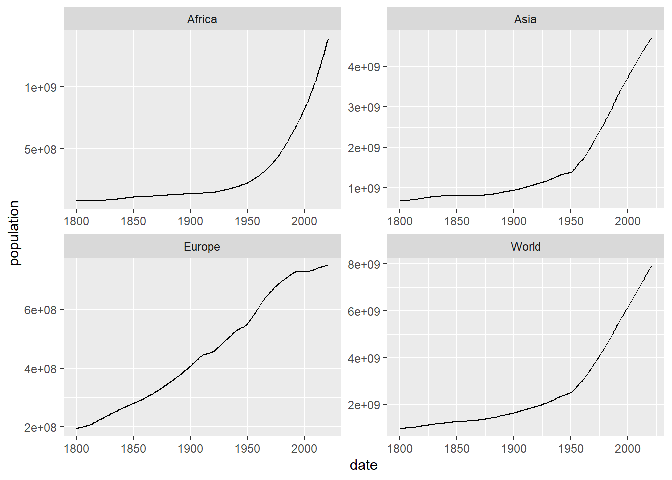
Figure 5.3: Separate drawing, in a grid, of the evolution of population in the world, Africa, Asia and Europe using facet_wrap
We can also compare the time series between them. The following table with graphs, built using the pivot_wider and ggpairs function of the GGally library, shows, on the diagonal, the density function of the distribution of values, at the bottom the scatterplot of each pair of time series and at the top the value of the correlation between each pair of time series, the closer that value is to 1, the better the combined values of each fit the regression line. We can observe that the evolution of the population in Europe has a different behavior than in the other regions, which produces a lower value of the correlation when comparing Europe with the other regions.
owid_population %>%
pivot_wider(values_from=population, names_from=location) |>
GGally::ggpairs(columns = 2:5)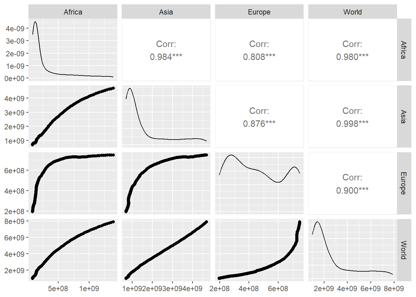
5.3 Seasonality
Many time series exhibit seasonality. For example, in a tourist location like the Canary Islands, the monthly movements of passengers at the airports depend on the month of the year, in accordance with the seasonal flows of tourists. In this case, our time series has a seasonality of 12, that is, our data are the monthly movements of passengers that we expect to present a similar (but not identical) behavior every 12 months. We are going to study the monthly passenger arrivals to the Canary Islands using a query made to ISTAC and stored in our local data folder.
istac_airports <- read.px("https://ctim.es/AEDV/data/istac_aeropuertos.px") %>%
as_tibble()
istac_airports
## # A tibble: 355 × 5
## Periodos Aeropuertos.de.origen Aeropuertos.de.destino Clases.de.tráfico
## <fct> <fct> <fct> <fct>
## 1 2020 Abril (p) TOTAL AEROPUERTOS DE… CANARIAS Regular
## 2 2020 Marzo (p) TOTAL AEROPUERTOS DE… CANARIAS Regular
## 3 2020 Febrero … TOTAL AEROPUERTOS DE… CANARIAS Regular
## 4 2020 Enero (p) TOTAL AEROPUERTOS DE… CANARIAS Regular
## 5 2019 TOTAL (p) TOTAL AEROPUERTOS DE… CANARIAS Regular
## 6 2019 Diciembr… TOTAL AEROPUERTOS DE… CANARIAS Regular
## 7 2019 Noviembr… TOTAL AEROPUERTOS DE… CANARIAS Regular
## 8 2019 Octubre … TOTAL AEROPUERTOS DE… CANARIAS Regular
## 9 2019 Septiemb… TOTAL AEROPUERTOS DE… CANARIAS Regular
## 10 2019 Agosto (… TOTAL AEROPUERTOS DE… CANARIAS Regular
## # ℹ 345 more rows
## # ℹ 1 more variable: value <dbl>We observe that in addition to monthly data, the TOTAL annual data appears in the table. We are going to remove these records, as well as the records that do not have an available value for passenger arrivals and the values for the year 2020 whose data is greatly affected by the COVID-19 epidemic.
istac_airports <- istac_airports %>%
filter(word(Periodos,2)!="TOTAL" & is.na(value)==FALSE & word(Periodos,1)!="2020")
istac_airports
## # A tibble: 252 × 5
## Periodos Aeropuertos.de.origen Aeropuertos.de.destino Clases.de.tráfico
## <fct> <fct> <fct> <fct>
## 1 2019 Diciembr… TOTAL AEROPUERTOS DE… CANARIAS Regular
## 2 2019 Noviembr… TOTAL AEROPUERTOS DE… CANARIAS Regular
## 3 2019 Octubre … TOTAL AEROPUERTOS DE… CANARIAS Regular
## 4 2019 Septiemb… TOTAL AEROPUERTOS DE… CANARIAS Regular
## 5 2019 Agosto (… TOTAL AEROPUERTOS DE… CANARIAS Regular
## 6 2019 Julio (p) TOTAL AEROPUERTOS DE… CANARIAS Regular
## 7 2019 Junio (p) TOTAL AEROPUERTOS DE… CANARIAS Regular
## 8 2019 Mayo (p) TOTAL AEROPUERTOS DE… CANARIAS Regular
## 9 2019 Abril (p) TOTAL AEROPUERTOS DE… CANARIAS Regular
## 10 2019 Marzo (p) TOTAL AEROPUERTOS DE… CANARIAS Regular
## # ℹ 242 more rows
## # ℹ 1 more variable: value <dbl>The word function allows us to extract the word, which occupies a certain position, from a string. Next we create a tsibble with the data. To construct the temporary variable we have to manipulate the date format used in this table by ISTAC to convert it to a standard date format and then convert it to a monthly date format.
istac_airports <- tsibble(
   date = paste(
           word(istac_airports$Periodos,1),
           word(istac_airports$Periodos,2),"1"
          ) %>%
         as.Date(format="%Y %B %d") %>% yearmonth(),
   passengers = istac_airports$value,
   index = date
)
istac_airports
## # A tsibble: 252 x 2 [1M]
## date passengers
## <mth> <dbl>
## 1 1999 ene. 117785
## 2 1999 feb. 120128
## 3 1999 mar. 130011
## 4 1999 abr. 140767
## 5 1999 may. 137081
## 6 1999 jun. 147560
## 7 1999 jul. 193930
## 8 1999 ago. 230282
## 9 1999 sep. 194375
## 10 1999 oct. 173292
## # ℹ 242 more rowsBelow we draw the time series where a clear seasonality can be observed.
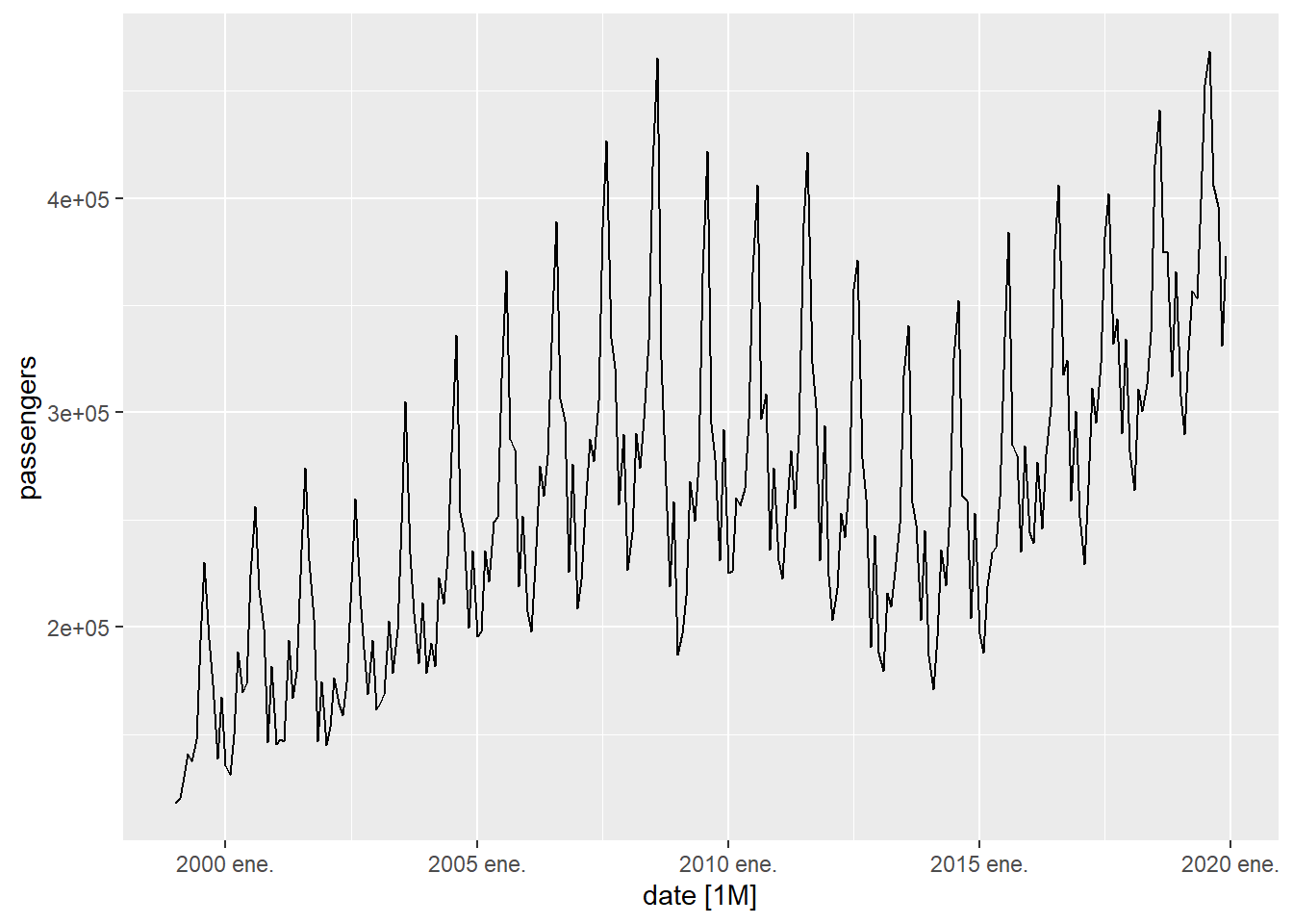
Figure 5.4: Evolution of passenger arrivals to the Canary Islands
Another interesting graph is to draw the time series separating it into 12-month periods. In this way it is clearly seen that the month with the most movement of travelers is August.
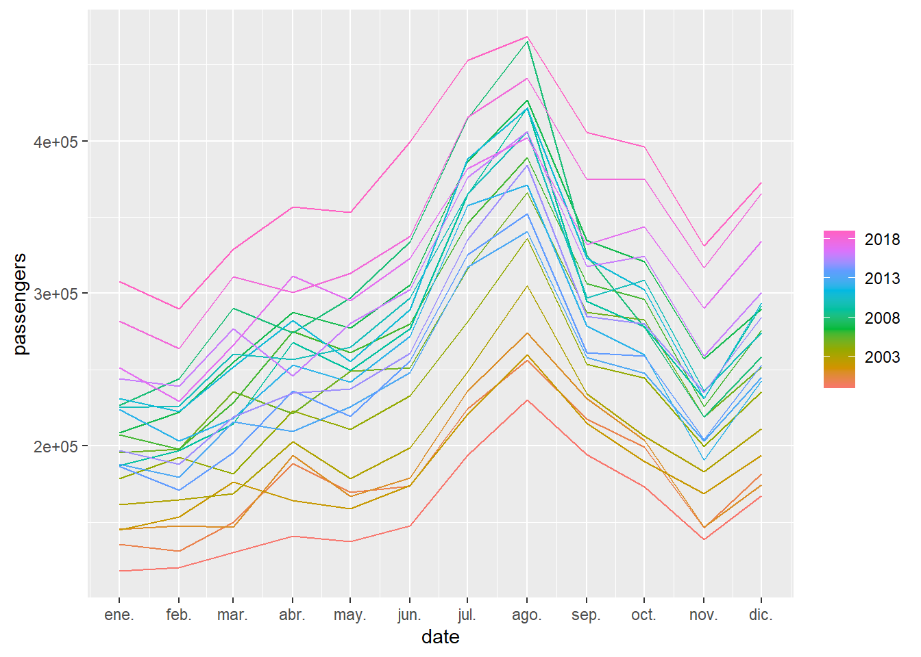
Figure 5.5: For the passenger arrival series to the Canary Islands, each annual series is represented as an independent curve
In the following graph it is separated by month and we see for each month how it evolves by year.
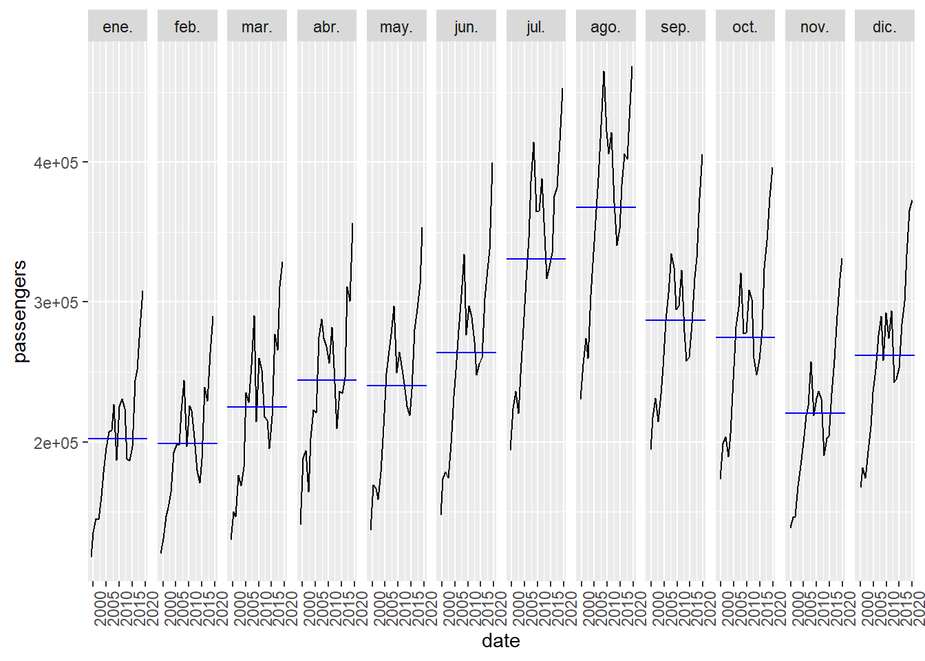
Figure 5.6: For the series of passenger arrivals to the Canary Islands, the evolution is represented by months
The following graph represents a scatter diagram with the observed variable, which we will call \(y_t\), with respect to the value of the same variable \(l\) months before \(y_{t-l}\). That is, for \(l=1\) (lag 1) the points \((y_{t},y_{t-1})\) are drawn. That is, we would be comparing the February data with the January data, the March data with February, etc. In this case, as we have a 12-month seasonality, we can observe that the point cloud \((y_{t},y_ {t-12})\) (lag 12) is the one that is most concentrated around the regression line that appears drawn. That is, when we compare the data for each month with the data for the same month of the previous year. One way to “guess” the seasonality of a time series would be to look at these graphs and see when the points are concentrated around the regression line.
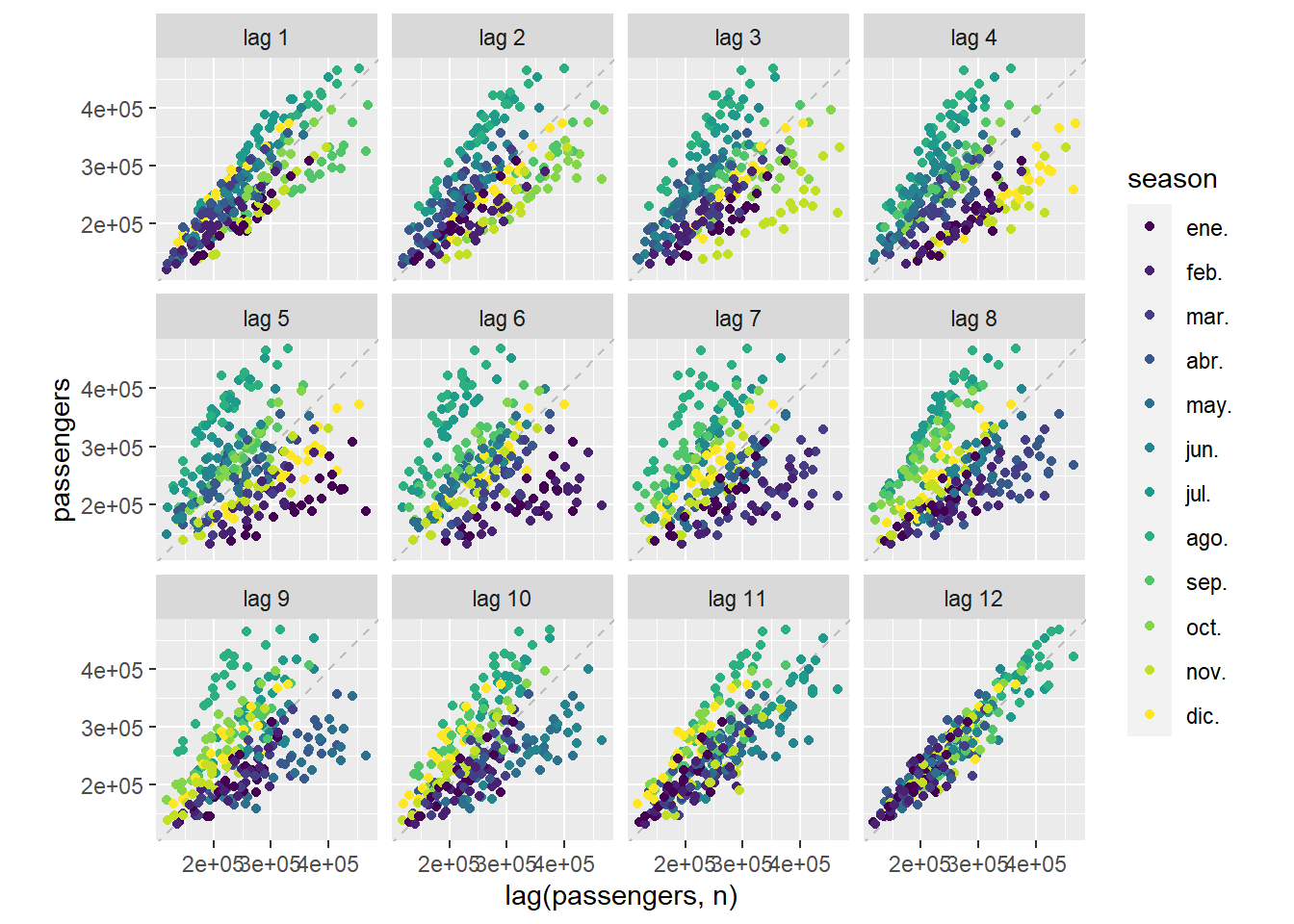
Figure 5.7: For the series of passenger arrivals to the Canary Islands \(y_t\), the points \((y_{t},y_{t-l})\) are represented
In some cases there may be a double seasonality. For example, if we study daily sales data in commerce, on the one hand they have a weekly seasonality, since sales depend on the day of the week and on the other hand they have an annual seasonality, because the annual period in which we are in may have a strong effect on sales, that is, for example, during the Christmas holidays more are sold than in other periods of the year. On the other hand, at the end of each month, companies usually accumulate late billing data, which produces an artificial peak in sales recorded on the last day of the month.
5.4 STL decomposition
A common way to manage the seasonality of a time series, which we denote by \(y_t\), is to use some model to extract the seasonality, which we denote by \(S_t\), and decompose the series as
\[ y_t = S_t + L_t + \mathcal{E}_t \] where \(L_t\) represents a trend curve of \(y_t\) freed from its seasonal component and \(\mathcal{E}_t\) represents the decomposition error committed by the model. A widely used model to obtain this decomposition is the so-called STL (“Seasonal and Trend decomposition using Loess”), which also allows managing double seasonality. We are going to apply, first of all, the STL method to decompose the time series of traveler arrivals to the Canary Islands:
istac_airports |>
   model(
     STL(passengers ~ season(period = 12),
     robust = TRUE)
   ) |>
   components() |>
   autoplot()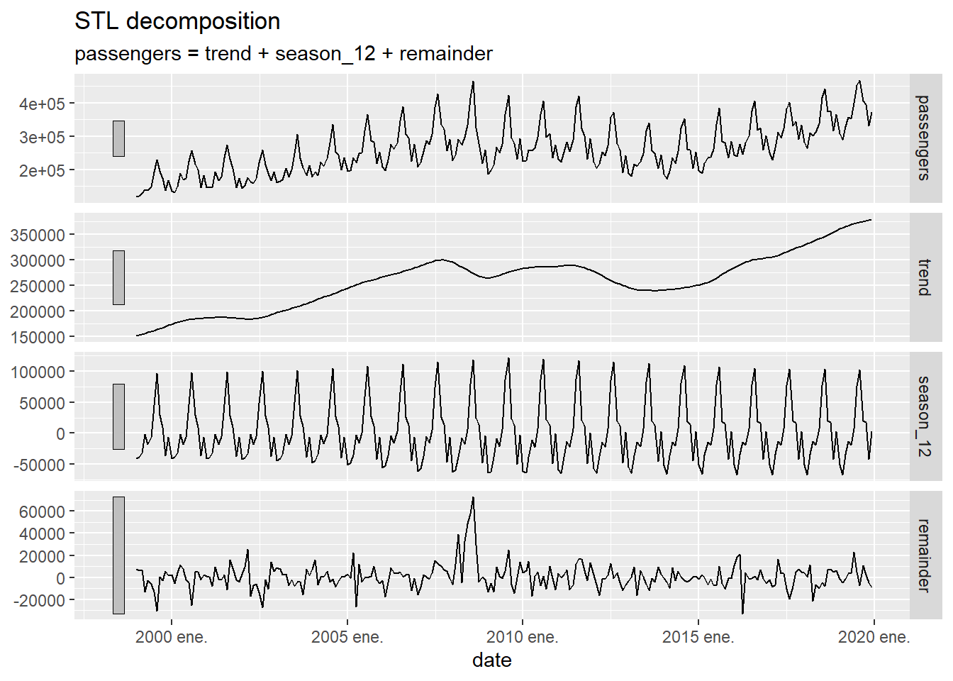
Figure 5.8: Decomposition of a time series using the STL method
The first graph presented is the original time series \(y_t\), the second is its smoothed version \(L_t\), the third is the seasonality \(S_t\) and the fourth is the model error \(\mathcal{E}_t\). For reasons of space and time, the mathematical foundation of the STL method, which can be found in CCMT90, will not be explained in this course.
To present an example with double seasonality, we are going to use the daily retail sales data of large companies in Spain published by the INE. Specifically, the original data used is the percentage of sales accumulated up to that day of the month, compared to the total sold the previous month. For example, the data for 03/15/2023 is 49.9, which represents that until that day of the month, 49.9% of what was sold in the entire previous month was sold. To better appreciate seasonality, instead of working with the accumulated data for the month, we are going to work with the daily data, that is, the percentage of sales each day, with respect to the total sales of the previous month. To obtain this data, it is enough to make the difference, each day, of the value accumulated that day with the value accumulated from the previous day.
# reading the INE table and managing dates
ine_accumulated_daily_trade <- read.xlsx("https://ctim.es/AEDV/data/ine_comercio_diario_acumulado.xlsx") %>%
   as_tibble() %>%
   mutate(date= as.Date(date,format = "%d/%m/%Y"))

  # creation of a tsibble with the data accumulated each month
  ine_accumulated_daily_trade <- tsibble(
   date = ine_accumulated_daily_trade$date,
   value = ine_accumulated_daily_trade$value,
   index = date
)

# creation of a tsibble with the difference of the data accumulated each month
ine_daily_trade <- ine_accumulated_daily_trade
for(i in 2:(length(ine_daily_trade$date)) ){
   if(format(ine_daily_trade$date[i],"%m") == format(ine_daily_trade$date[i-1],"%m")){
     ine_daily_trade$value[i]=ine_accumulated_daily_trade$value[i]-ine_accumulated_daily_trade$value[i-1]
   }
}
To illustrate double seasonality we are going to draw the time series ine_daily_trade in a period of 3 months. Where you can see the weekly seasonality (the highest sales correspond to Fridays and Saturdays and the lowest to Sundays) and the annual seasonality (every year in December more are sold, then sales decrease from the second week of January and begin to up in March). Furthermore, at the end of each month there is a strong rebound in recorded sales because, due to the accounting system that many companies use, more sales are recorded on the last day of each month.
  ine_daily_trade %>%
    filter(date>= as.Date("2022-12-15") & date<= as.Date("2023-03-15")) %>%
    autoplot(value)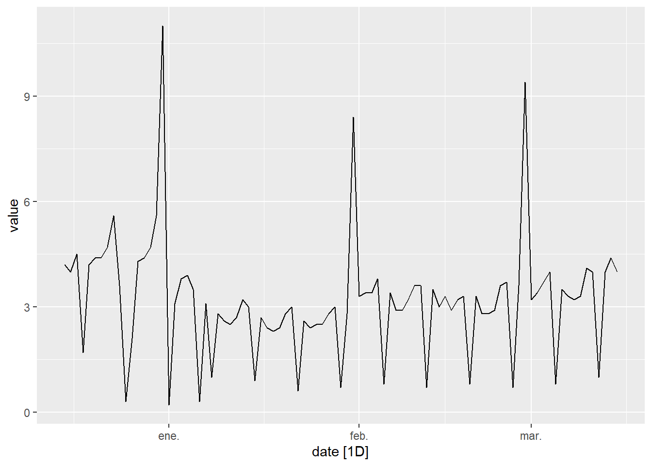
Figure 5.9: Commerce sales data in Spain in a period of 3 months
Next we are going to apply the STL method to decompose the ine_comercio_daily time series. We observe that a weekly and an annual seasonality appears. In view of the evolution of the trend curve, it is observed how sales have been decreasing since 2020 (a behavior that is not visible when observing the original data).
ine_daily_trade %>% model(
   STL(value ~ season(period = 7) +
                     season(period = 365.25),
       robust = TRUE)
) %>%
   components() |>
   autoplot()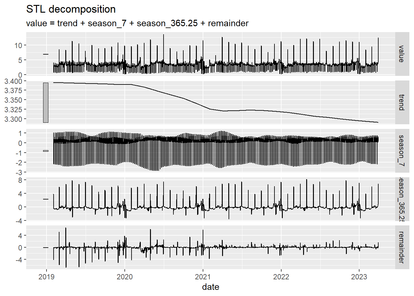
Figure 5.10: Calculation of STL decomposition with double seasonality
5.5 Prediction
A fundamental aspect of time series analysis is making predictions of the future value of the time series based on the values we know. To do this, it is necessary to use mathematical prediction models. Here we are going to briefly introduce two of the most used models, such as exponential smoothing and ARIMA models. In general, we will denote by \(y_t\) the observed value of the time series at time \(t\) and by \(\hat y_{t+h|t}\) the value that the model predicts for time \(t+h\) using the data observed up to instant \(t\). Furthermore, we will study how these models can be applied to the case of double seasonality.
5.6 Exponential smoothing
We are going to introduce this predictive model progressively, starting with its simplest version and later adding new features to the model.
simple model
The simplest version of this model is given by
\[\hat y_{t+1|t} = \alpha y_t + (1-\alpha) \hat y_{t|t-1},\] is a recursive prediction model where the prediction value is an average weighted by the variable \(\alpha\) between the value observed the previous day and the model’s prediction for the previous day. Starting the iterations from the beginning we would have:
\[ \hat y_{2|1} = \alpha y_1 + (1-\alpha) l_0\\ \hat y_{3|2} = \alpha y_2 + (1-\alpha) \hat y_{2|1}=\alpha y_2+(1-\alpha)\alpha y_1 + (1-\alpha)^2 l_0\\ \hat y_{4|3} = \alpha y_3 + (1-\alpha) \hat y_{3|2}= \alpha y_3+\alpha(1-\alpha) y_2+(1-\alpha)^2\alpha y_1 + (1-\alpha)^3 l_0\\ ........\]
Since the value \(y_{1|0}\) does not exist, it is replaced by \(l_0\) which is a parameter of the model along with the value of \(\alpha\). In practice, to calculate the parameters of a model, a prediction error between the estimated values and the observed values is minimized. From the previous equations, we observe that the value of \(\hat y_{t+1|t}\) can be expressed as a weighted average of all previous values of \(y_t\) where the weight of each term declines as we go into the past. This behavior is what gives it its name to this prediction method (exponential smoothing).
Smoothing and trending
The following version of this model introduces the variable \(b_t\) (the slope or trend), and \(l_t\) which determines the smoothed value of the time series:
\[ l_t = \alpha y_t +(1-\alpha)(l_{t-1}+b_{t-1})\\ b_t = \beta^*(l_t -l_{t-1})+(1-\beta^*)b_{t-1}\\ \hat y_{t+h|t}=l_t+hb_t, \] This model is projected into the future using a straight line, therefore, it will fit well to time series that vary linearly. This model will have as parameters \(\alpha\), \(l_0\), \(\beta^*\) and \(b_0\).
Damped model
To fit better non-linear time series, an additional parameter \(\phi\) can be introduced that allows the prediction to be “damped” using the following modification of the model:
\[ l_t = \alpha y_t +(1-\alpha)(l_{t-1}+\phi b_{t-1})\\ b_t = \beta^*(l_t -l_{t-1})+(1-\beta^*)\phi b_{t-1}\\ \hat y_{t+h|t}=l_t+(\phi+\phi^2+\cdots+\phi^h)b_t, \]
Seasonality
To take seasonality into account, a new series \(s_t\) is introduced. Seasonality can be introduced multiplicatively or additively in the following way:
\[ \text{multiplicative seasonality : } \hat y_{t+h|t}=(l_t+(\phi+\phi\cdots+\phi^h)b_t)*s_{t-m+h\%m} \\ \text{additive seasonality : } \hat y_{t+h|t}=l_t+(\phi+\cdots+\phi^h)b_t +s_{t-m+h\%m} \]
where \(m\) is the period of the seasonality (for example \(m=12\) for a monthly seasonality) and \(h\%m\) is the remainder of the division between \(h\) and \(m\). In this way, seasonality extends into the future periodically, with period \(m\). Seasonality also affects the other equations of the model, let’s see how the model would look for additive seasonality:
\[ l_t = \alpha (y_t -s_{t-m})+(1-\alpha)(l_{t-1}+b_{t-1})\\ b_t = \beta^*(l_t -l_{t-1})+(1-\beta^*)b_{t-1}\\ s_t=\gamma(y_t-l_{t-1}-b_{t-1})+(1-\gamma)s_{t-m}\\ \hat y_{t+h|t}=l_t+hb_t+s_{t-m+h\%m}, \] In the case of multiplicative seasonality the model would be
\[ l_t = \alpha \frac{y_t}{s_{t-m}}+(1-\alpha)(l_{t-1}+b_{t-1})\\ b_t = \beta^*(l_t -l_{t-1})+(1-\beta^*)b_{t-1}\\ s_t=\gamma\frac{y_t}{l_{t-1}+b_{t-1})}+(1-\gamma)s_{t-m}\\ \hat y_{t+h|t}=(l_t+hb_t)s_{t-m+h\%m}, \]
To analyze the error, \(\varepsilon_t\), which is committed between the value predicted by the model and the observed value, additive or multiplicative error models can also be used. That is, given an observed value, \(y_t\), and its approximation by the model \(\hat y_{t|t-1}\), the error \(\varepsilon_t\) can be defined in the following ways:
\[ \text{additive error : } y_t=\hat y_{t|t-1}+\varepsilon_t\\ \text{multiplicative error : } y_t=\hat y_{t|t-1}(1+\varepsilon_t) \]
Optimal estimate
As can be seen, this model presents a variety of options. To bring together this information, the ETS notation is used (Error Option, Trend Option, Seasonality Option). Regarding the error (the E in the ETS string), the model can be additive (A) or multiplicative (M), with respect to the trend (the T in the ETS string), it may have no trend (N), with a simple trend (A) or with a damped trend (A\(_d\)), with respect to seasonality (the S in the ETS string) it can be without seasonality (N) with additive seasonality (A) or with multiplicative seasonality (M). For example, an ETS(M,A,N) model would be a model with multiplicative error, simple trend and without seasonality. Fortunately, we do not need to decide which model to choose and calculate the optimal values of its parameters, we can use the model function of the fpp3 library that automatically calculates the best model and parameters that fit our time series. For example, let’s calculate the best model that fits the world population data series:
## Series: population
## Model: ETS(M,A,N)
##   Smoothing parameters:
##     alpha = 0.8635692
##     beta  = 0.708906
##
##   Initial states:
##       l[0]    b[0]
##  980810630 4967560
##
##   sigma^2:  0
##
##      AIC     AICc      BIC
## 7864.834 7865.112 7881.847
We observe that for this time series the best model is ETS(M,A,N), that is multiplicative error, simple trend and no seasonality. Furthermore we see how the function has calculated the optimal parameters of the model. The values of AIC, AICc and BIC are indicators of the quality of the model fit to the time series, The smaller these values are, the better the fit will be. These fit quality indicators also take into account the number of optimized parameters in the model. The greater the number of parameters, the worse the model is considered since the phenomenon called “overfitting” can occur, which is that if there are many parameters, the model can fit very well to the sample data, since we handle many degrees of freedom, but it can fail greatly in new data that has not been considered in the adjustment (as is the case of prediction in the future). Once the fit model has been calculated, we will use it to make a prediction of the world population 20 years ahead using the ‘forecast’ function
## # A fable: 20 x 5 [1Y]
## # Key:     location, .model [1]
##    location .model           date          population       .mean
##    <chr>    <chr>           <dbl>              <dist>       <dbl>
##  1 World    ETS(population)  2022   N(8e+09, 1.5e+14) 7980988418.
##  2 World    ETS(population)  2023 N(8.1e+09, 5.1e+14) 8051332443.
##  3 World    ETS(population)  2024 N(8.1e+09, 1.3e+15) 8121676467.
##  4 World    ETS(population)  2025 N(8.2e+09, 2.6e+15) 8192020492.
##  5 World    ETS(population)  2026 N(8.3e+09, 4.7e+15) 8262364517.
##  6 World    ETS(population)  2027 N(8.3e+09, 7.6e+15) 8332708541.
##  7 World    ETS(population)  2028 N(8.4e+09, 1.2e+16) 8403052566.
##  8 World    ETS(population)  2029 N(8.5e+09, 1.7e+16) 8473396591.
##  9 World    ETS(population)  2030 N(8.5e+09, 2.3e+16) 8543740615.
## 10 World    ETS(population)  2031 N(8.6e+09, 3.2e+16) 8614084640.
## 11 World    ETS(population)  2032 N(8.7e+09, 4.1e+16) 8684428665.
## 12 World    ETS(population)  2033 N(8.8e+09, 5.3e+16) 8754772689.
## 13 World    ETS(population)  2034 N(8.8e+09, 6.7e+16) 8825116714.
## 14 World    ETS(population)  2035 N(8.9e+09, 8.3e+16) 8895460739.
## 15 World    ETS(population)  2036     N(9e+09, 1e+17) 8965804763.
## 16 World    ETS(population)  2037   N(9e+09, 1.2e+17) 9036148788.
## 17 World    ETS(population)  2038 N(9.1e+09, 1.5e+17) 9106492812.
## 18 World    ETS(population)  2039 N(9.2e+09, 1.7e+17) 9176836837.
## 19 World    ETS(population)  2040   N(9.2e+09, 2e+17) 9247180862.
## 20 World    ETS(population)  2041 N(9.3e+09, 2.4e+17) 9317524886.
The .mean variable tells us the prediction value and the population variable tells us
indicates the probability distribution of the expected value. This distribution
allows us to calculate confidence intervals, which are of great importance for studying the
expected range of values in which our prediction moves. For example, in the previous case, for the year 2022, the model predicts that the world population follows a normal distribution of mean \(\mu=8 \cdot 10^9\) and variance \(\sigma^2=1.5 \cdot 10^ {14}\). Taking into account that it is a normal distribution, the confidence intervals have the form \([\mu-c \cdot \sigma,\mu+c\cdot \sigma]\) where \(c\) depends on the desired percentage. For example, for the confidence interval at \(80\%\), we have \(c=1.28\), and for the confidence interval at \(95\%\), \(c=1.96\). In particular, in our example of the world population for the year 2022, the confidence interval at \(95\%\) is
\[ [8 \cdot 10^9-1.96\sqrt{1.5 \cdot 10^{14}},8 \cdot 10^9+1.96\sqrt{1.5 \cdot 10^{14}}] \] It is important to note that the calculation of these confidence intervals assumes that the residuals (errors) of the prediction model follow an uncorrelated normal distribution with constant variance that is maintained in the future (uncorrelated means that the error at a time instant in the series does not depend on the error at other time instants). In particular, if the conditions that determine the evolution of the time series change greatly in the future, the real value of the time series may be very far from the calculated confidence interval. For example, an event such as the lockdown during the COVID-19 epidemic renders predictions made in the past for that period completely useless for many time series such as the expected number of passengers traveling by plane.
The following graph shows the observed value of the population after the year 2000 and the prediction with the confidence intervals around it (confidence levels of 80% and 95%). A 80% confidence interval means that in 80% of the cases the real value of the population will be found within the interval (represented by the dark blue band). It can be observed that, as expected, the further we go into the future, the larger the size of the confidence interval because the degree of uncertainty is greater.
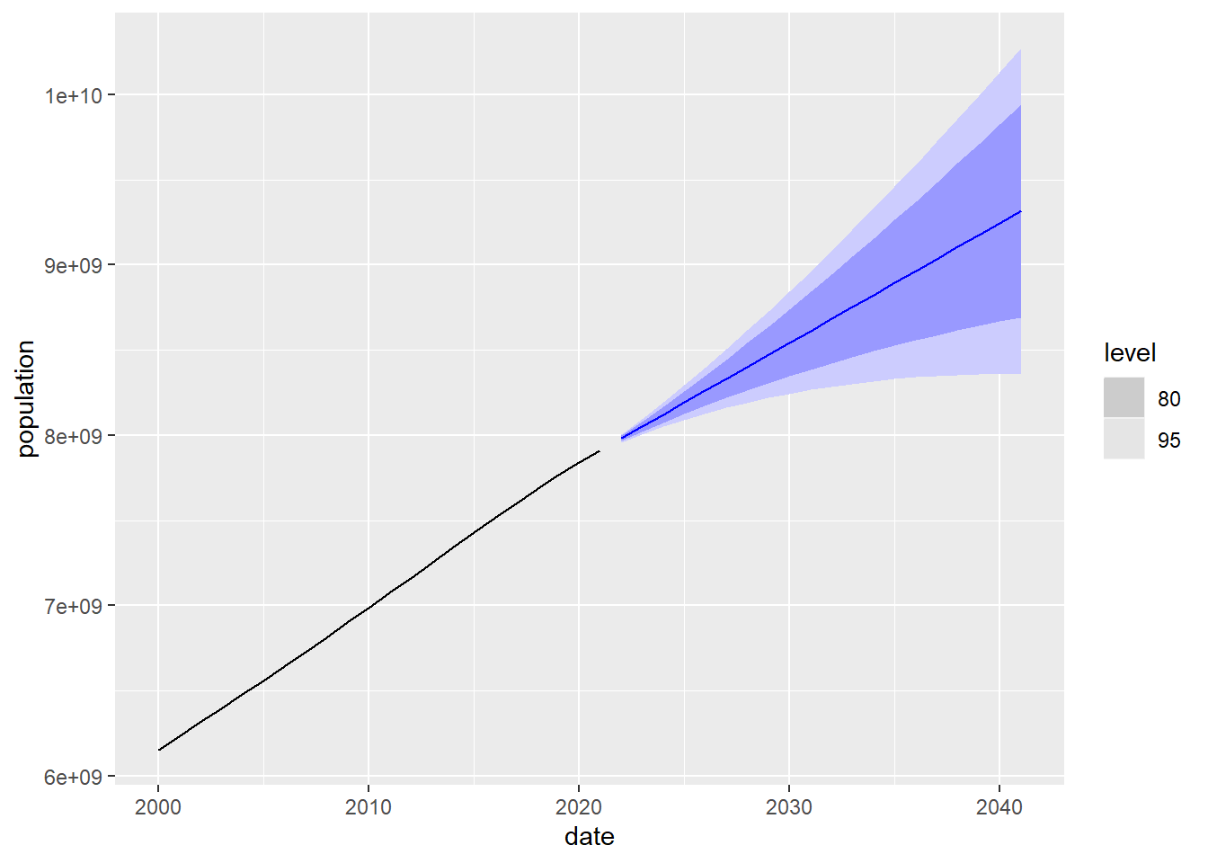
Figure 5.11: 20-year prediction of world population using the exponential smoothing model
Now we will repeat the process with the time series of traveler arrivals to Canary Islands, which is a time series with seasonality. We observe that in this case the best model is of the type ETS(M,A,M), which corresponds to a series with multiplicative seasonality. Furthermore, in this case the prediction fails completely. due to the enormous impact that the COVID epidemic had on passenger movement. This tells us that predictive models, like the ones studied here, are based in which the factors that condition the evolution of the time series will be the same in the future than in the past. When events occur that modify these factors of evolution, the reliability of the prediction can deteriorate greatly.
## Series: passengers
## Model: ETS(M,A,M)
##   Smoothing parameters:
##     alpha = 0.541925
##     beta  = 0.002598776
##     gamma = 0.09755761
##
##   Initial states:
##    l[0]     b[0]      s[0]     s[-1]    s[-2]    s[-3]    s[-4]    s[-5]
##  145152 1894.426 0.9742414 0.8335583 1.053734 1.134229 1.412889 1.244848
##      s[-6]     s[-7]     s[-8]     s[-9]    s[-10]    s[-11]
##  0.9980586 0.9339813 0.9840955 0.8667885 0.7843986 0.7791779
##
##   sigma^2:  0.0032
##
##      AIC     AICc      BIC
## 6227.709 6230.325 6287.710
Note that in the ETS model, when there is seasonality of period \(m\), the number of parameters can increase greatly since, in addition to the parameter \(\gamma\), \(m-1\) parameters are required to control the initial values of \(s_t\) .
## # A fable: 24 x 4 [1M]
## # Key:     .model [1]
##    .model               date         passengers   .mean
##    <chr>               <mth>             <dist>   <dbl>
##  1 ETS(passengers) 2020 ene.  N(3e+05, 2.9e+08) 302411.
##  2 ETS(passengers) 2020 feb. N(291356, 3.5e+08) 291356.
##  3 ETS(passengers) 2020 mar. N(334528, 5.7e+08) 334528.
##  4 ETS(passengers) 2020 abr. N(361755, 7.9e+08) 361755.
##  5 ETS(passengers) 2020 may. N(361928, 9.1e+08) 361928.
##  6 ETS(passengers) 2020 jun.  N(4e+05, 1.2e+09) 396892.
##  7 ETS(passengers) 2020 jul. N(490388, 2.1e+09) 490388.
##  8 ETS(passengers) 2020 ago. N(539218, 2.9e+09) 539218.
##  9 ETS(passengers) 2020 sep.   N(430142, 2e+09) 430142.
## 10 ETS(passengers) 2020 oct. N(417467, 2.1e+09) 417467.
## # ℹ 14 more rows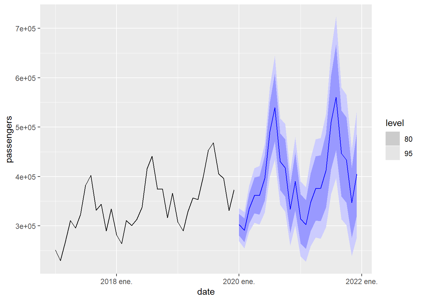
Figure 5.12: 2-year prediction of passenger arrivals in the Canary Islands using the exponential smoothing model
This exponential smoothing model decomposes the time series using \(l_t\) (a smoothed version of the time series), \(b_t\) (the slope), \(s_t\) (the seasonality) and the error ( remainder), which, being multiplicative, is expressed as \(1+\varepsilon_t\) . The following graph illustrates this decomposition:
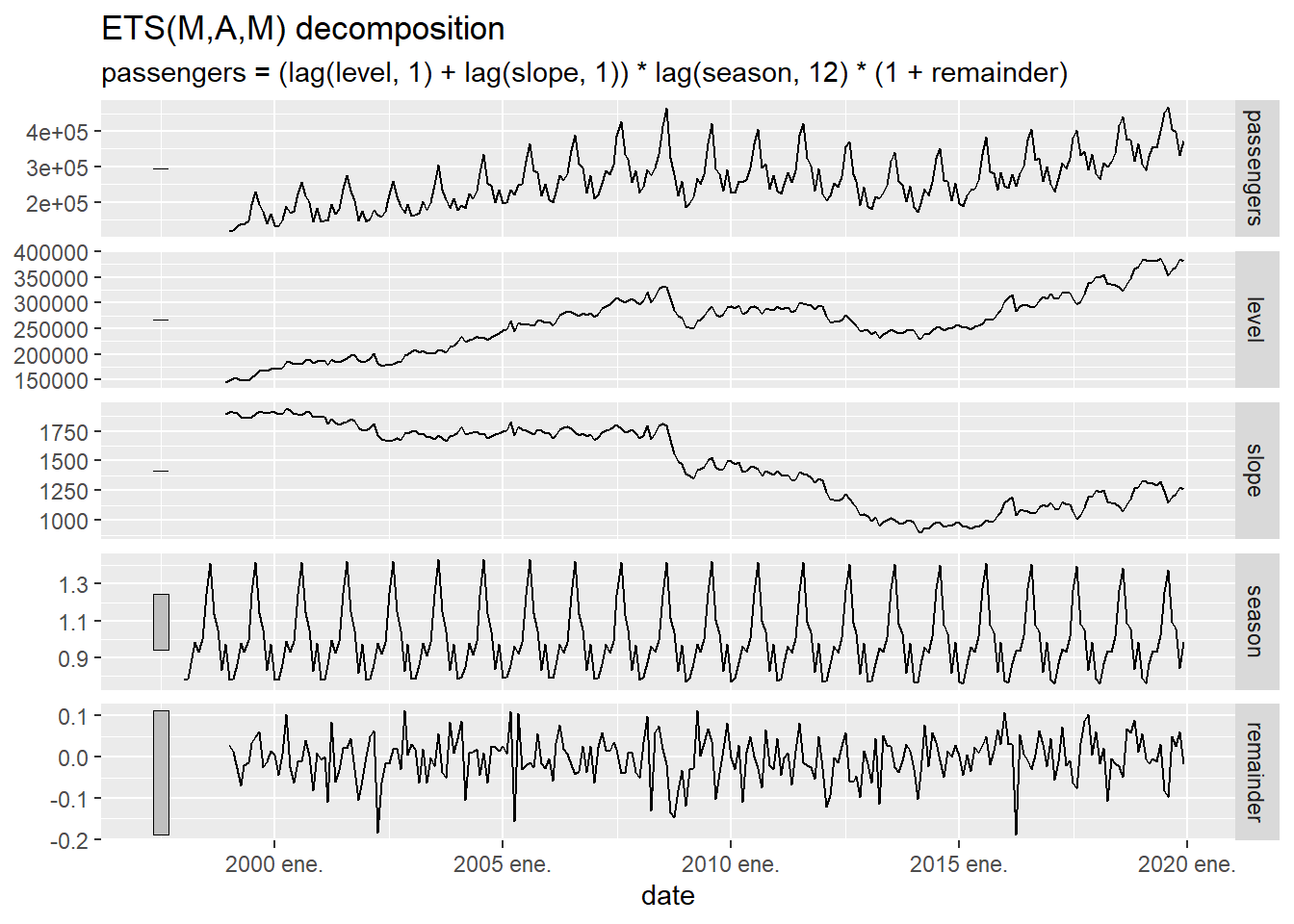
Figure 5.13: Decomposition of the time series of arrivals at the Canary Islands airports using the exponential smoothing model.
Double seasonality management
This model is not designed to directly manage double seasonality. An alternative way to proceed to manage seasonality is to use the STL decomposition of the time series, apply the exponential smoothing model without seasonality to predict the value of the trend curve \(L_t\) obtained in the STL decomposition and predict the value of \(y_t\) from that prediction also using a periodic extension of the seasonality \(S_t\) calculated by the STL decomposition. This allows us to combine seasonalities with different periods. Next we are going to apply this procedure to the time series ine_daily_trade:
# STL decomposition application combined with ETS without seasonality
fit <- decomposition_model(
   STL(value ~ season(period = 7) + # we add weekly seasonality
               season(period = 365.25), # add annual seasonality
       robust = TRUE),
   ETS(season_adjust ~ season("N")) # ETS model calculation without seasonality
)
# Calculation and drawing prediction one year ahead
ine_daily_trade %>%
   model(fit) %>%
   forecast(h =365) %>%
   autoplot( ine_daily_trade%>%
              filter(date>= as.Date("2022-01-01"))
           )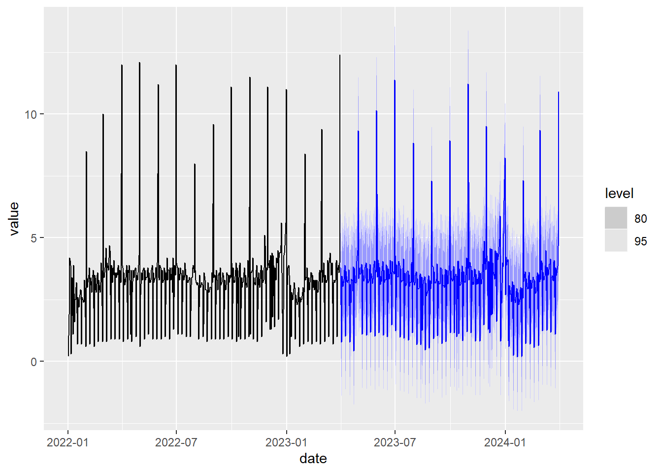
Figure 5.14: Prediction using STL decomposition and exponential smoothing.
5.7 The ARIMA model
Autoregressive model (AR)
The simplest version of the ARIMA prediction model is the so-called autoregressive model (AR) where each observed value \(y_t\) is approximated by a linear combination of previously observed values, that is:
\[ y_t = c + \phi_1 y_{t-1}+\phi_2 y_{t-2}+ \cdots +\phi_p y_{t-p}+ \varepsilon_t \] where \(p\) represents the number of values in the past that are taken to approximate the value of \(y_t\), and \(\varepsilon_t\) is the approximation error. \(c\) and \(\phi_1,...,\phi_p\) are the model parameters. We are going to express this equation by introducing the time shift operator, \(B\):
\[ By_t = y_{t-1} \] Using the \(B\) operator we can write the AR model equation as:
\[ (1-\phi_1B-\phi_2B^2-\cdots\phi_pB^p)y_t = c + \varepsilon_t \]
Derivatives
For the AR model to work well, the time series should not have a defined trend of growth or decrease. The usual way to remove the trend of a time series is to use some derivative of the time series in the model instead of the time series itself. The first derivative is defined as:
\[ (1-B)y_t=y_t-y_{t-1}. \] The second derivative would be the derivative of the derivative, that is:
\[ (1-B)^2y_t=(1-B)(y_t-y_{t-1})=y_t-y_{t-1} -(y_{t-1}-y_{t-2})=y_t-2y_{t-1}+y_{t-2}. \] Therefore, with this notation, the derivative of order \(d\) would be \((1-B)^dy_t\). When calculating the derivatives of a time series, it loses its trend. To illustrate this, in the following graphs we show the time series of the world population and its first 3 derivatives. As can be seen, in the third derivative the time series no longer has a defined growth pattern.
p1 <- owid_population %>%
   filter(location=="World") %>%
   autoplot(population)
data <- owid_population %>%
filter(location=="World")
data$derivative_1 <- derivada(data$population)
p2 <- data %>% autoplot(derivative_1)
data$derivative_2 <- derivada(data$derivative_1)
p3 <- data %>% autoplot(derivative_2)
data$derivative_3 <- derivada(data$derivative_2)
p4 <- data %>% autoplot(derivative_3)
wrap_plots(p1, p2, p3, p4, ncol = 2, nrow = 2)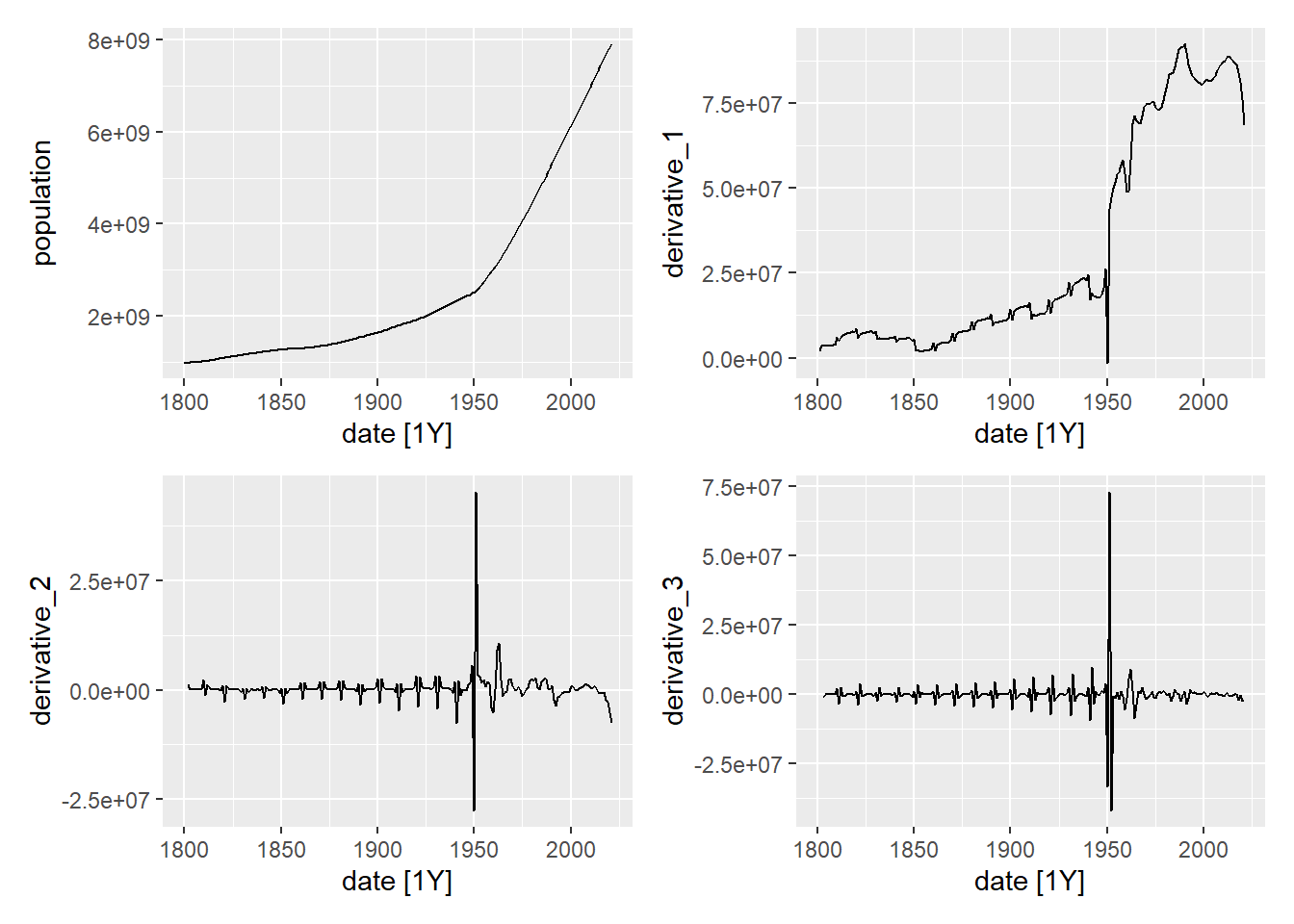
Figure 5.15: Time series of world population and its derivatives
By replacing the original series in the model (AR) with its derivative of order d, we obtain the model
\[ (1-\phi_1B-\phi_2B^2-\cdots-\phi_pB^p)(1-B)^dy_t = c + \varepsilon_t \] where the order, \(d\), of the derivative used appears as an additional parameter.
ARIMA(p,d,q)
Next, to improve the model, we add a linear combination of past errors (this part of the model is called (MA)), arriving at the non-seasonal ARIMA model given by: \[ (1-\phi_1B-\cdots\phi_pB^p)(1-B)^dy_t = c + \varepsilon_t + \theta_1\varepsilon_{t-1}+\cdots \theta_q\varepsilon_{t-q} \] which can also be expressed as:
\[ (1-\phi_1B-\cdots-\phi_pB^p)(1-B)^dy_t = c + (1 + \theta_1B+\cdots \theta_qB^q)\varepsilon_{t} \] This model is called ARIMA(p,d,q). Defining the functions
\[ \phi(B)=1-\phi_1B-\cdots-\phi_pB^p \\ \theta(B)=1 + \theta_1B+\cdots \theta_qB^q \] The ARIMA(p,d,q) model can be expressed more compactly as
\[ \phi(B)(1-B)^dy_t=c+\theta(B)\varepsilon_{t} \]
ARIMA(p,d,q)(P,D,Q)\(_m\)
To introduce a period seasonality \(m\) in the ARIMA model, we use the \(m\) spaced time series given by \(y_t,y_{t-m},y_{t-2m},y_{t-3m},..\) that can be expressed as \(y_t,B^my_t,B^{2m}y_t,B^{3m}y_t,..\). Let’s consider the new functions:
\[ \Phi(B^m)=1-\Phi_1B^m-\cdots-\Phi_PB^{mP} \\ \Theta(B^m)=1 + \Theta_1B^m+\cdots \Theta_QB^{mQ} \]
Using this notation, the application of the ARIMA model to the \(m\) spaced time series can be expressed as :
\[ \Phi(B^m)(1-B^m)^Dy_t=c+\Theta(B^m)\varepsilon_{t} \]
The general ARIMA model with seasonality \(m\) is denoted as ARIMA(p,d,q)(P,D,Q)\(_m\) and is defined by the following combination of the application of the above model to the original time series and to the \(m\) spaced time series:
\[ \phi(B)\Phi(B^m)(1-B)^d(1-B^m)^Dy_t=c+\theta(B)\Theta(B^m)\varepsilon_{t} \]
Prediction with ARIMA
To make predictions in the future using the ARIMA model we solve \(y_t\) from the model equation and we are left with
\[ y_t=c+\left(1-\phi(B)\Phi(B^m)(1-B)^d(1-B^m)^D\right)y_t+\theta(B)\Theta(B^m)\varepsilon_{t} \] As the model is constructed, the second part of the equality is a linear combination of values prior to \(y_t\), that is, \(y_{t-1},y_{t-2},...,\), but no of \(y_t\) and a linear combination of values of \(\varepsilon_t\). If \(y_T\) is the last known value of \(y_t\), then the last value we can calculate from the observed error is \(\varepsilon_T\). In the prediction formula, we will always consider that \(\varepsilon_t=0\) for \(t>T\). We can then define the prediction \(\hat y_{T+1|T}\) as
\[ \hat y_{T+1|T}=c+\left(1-\phi(B)\Phi(B^m)(1-B)^d(1-B^m)^D\right)y_{T+1}+\theta(B)\Theta(B^m)\varepsilon_{T+1} \]
The right side of the equation can be evaluated with the known data because, as stated above, only values of \(y_t\) are involved with \(t\leq T\) and we assign \(\varepsilon_{T+1}=0\). Now we recursively apply the formula to obtain the prediction at later times taking as previous values of \(y_t\) those observed (for \(t \leq T\)) and those predicted by the model for (\(t>T\)). In the same way \(\varepsilon_t\) will be the observed value for \(t \leq T\) and 0 for \(t>T\). For example, to calculate \(\hat y_{T+2|T}\) you use \(y_{t+1}=\hat y_{T+1|T}\) to the right of the equation and \(\varepsilon_{T+ 2}=0\).
Optimal estimate
As in the case of exponential smoothing models, to automatically calculate the model
optimal ARIMA for a time series we will use the model function that supplies
the library. This function may take some time to execute
fit <- owid_population %>%
   filter(location=="World") %>%
   model(ARIMA(population,stepwise = FALSE, approx = FALSE))
report(fit)
## Series: population
## Model: ARIMA(2,2,4)
##
## Coefficients:
## ar1 ar2 ma1 ma2 ma3 ma4
## 1.0186 -0.8519 -1.366 1.3471 -0.3992 0.1736
## s.e. 0.0742 0.0686 0.098 0.1454 0.1330 0.0855
##
## sigma^2 estimated as 1.444e+13: log likelihood=-3642.69
## AIC=7299.37 AICc=7299.9 BIC=7323.13We observe that the resulting model is an ARIMA(2,2,4) without seasonality. Looking the coefficients the resulting model would be
\[ (1-1.0186B+0.8519B^2)(1-B)^2y_t=\varepsilon_{t} -1.366\varepsilon_{t-1} + 1.3471\varepsilon_{t-2} - 0.3992\varepsilon_{t-3} + 0.1736\varepsilon_{t-4} \] The values of AIC, AICc and BIC are slightly lower than those obtained using the exponential smoothing model and therefore, for this time series the model that best fits is the ARIMA.
Next we are going to make a 20-year prediction of the world population 20 years from now. We note that the exponential smoothing model previously applied to this series predicts a population of 9.317 billions by 2041 and the ARIMA model predicts 9.26 billions.
## # A fable: 20 x 5 [1Y]
## # Key:     location, .model [1]
##    location .model                               date          population  .mean
##    <chr>    <chr>                               <dbl>              <dist>  <dbl>
##  1 World    ARIMA(population, stepwise = FALSE…  2022   N(8e+09, 1.4e+13) 7.98e9
##  2 World    ARIMA(population, stepwise = FALSE…  2023   N(8e+09, 5.4e+13) 8.05e9
##  3 World    ARIMA(population, stepwise = FALSE…  2024 N(8.1e+09, 1.4e+14) 8.12e9
##  4 World    ARIMA(population, stepwise = FALSE…  2025   N(8.2e+09, 3e+14) 8.18e9
##  5 World    ARIMA(population, stepwise = FALSE…  2026 N(8.2e+09, 5.5e+14) 8.25e9
##  6 World    ARIMA(population, stepwise = FALSE…  2027 N(8.3e+09, 9.4e+14) 8.32e9
##  7 World    ARIMA(population, stepwise = FALSE…  2028 N(8.4e+09, 1.5e+15) 8.38e9
##  8 World    ARIMA(population, stepwise = FALSE…  2029 N(8.5e+09, 2.2e+15) 8.45e9
##  9 World    ARIMA(population, stepwise = FALSE…  2030 N(8.5e+09, 3.1e+15) 8.52e9
## 10 World    ARIMA(population, stepwise = FALSE…  2031 N(8.6e+09, 4.2e+15) 8.59e9
## 11 World    ARIMA(population, stepwise = FALSE…  2032 N(8.7e+09, 5.6e+15) 8.65e9
## 12 World    ARIMA(population, stepwise = FALSE…  2033 N(8.7e+09, 7.2e+15) 8.72e9
## 13 World    ARIMA(population, stepwise = FALSE…  2034 N(8.8e+09, 9.1e+15) 8.79e9
## 14 World    ARIMA(population, stepwise = FALSE…  2035 N(8.9e+09, 1.1e+16) 8.85e9
## 15 World    ARIMA(population, stepwise = FALSE…  2036 N(8.9e+09, 1.4e+16) 8.92e9
## 16 World    ARIMA(population, stepwise = FALSE…  2037   N(9e+09, 1.7e+16) 8.99e9
## 17 World    ARIMA(population, stepwise = FALSE…  2038   N(9.1e+09, 2e+16) 9.06e9
## 18 World    ARIMA(population, stepwise = FALSE…  2039 N(9.1e+09, 2.4e+16) 9.12e9
## 19 World    ARIMA(population, stepwise = FALSE…  2040 N(9.2e+09, 2.8e+16) 9.19e9
## 20 World    ARIMA(population, stepwise = FALSE…  2041 N(9.3e+09, 3.3e+16) 9.26e9
Let’s now draw the prediction using the ARIMA model with the intervals of confidence together with the series observed since 2000. Visually we observe that the confidence intervals are smaller than those in the graph for the ETS model, which also indicates a better fit of the ARIMA model.
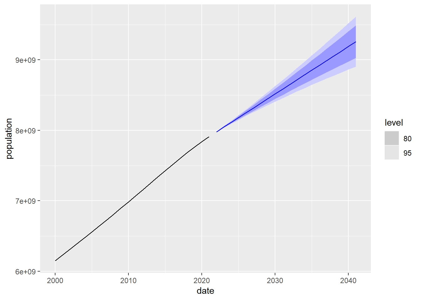
Figure 5.16: 20-year prediction of world population using the ARIMA model
Next we apply the ARIMA model to the study of the time series of the arrival of travelers to the Canary Islands.
## Series: passengers
## Model: ARIMA(1,0,1)(2,1,1)[12] w/ drift
##
## Coefficients:
##          ar1      ma1     sar1     sar2    sma1   constant
##       0.9456  -0.3465  -1.0375  -0.5581  0.4769  1506.8730
## s.e.  0.0233   0.0741   0.0912   0.0602  0.0992   831.2594
##
## sigma^2 estimated as 198330585:  log likelihood=-2634.69
## AIC=5283.38   AICc=5283.86   BIC=5307.74
We note that in this case an ARIMA(1,0,1)(2,1,1)\(_{12}\) model is obtained. Starting From the estimated parameters it is obtained that the model is given by
\[ (1-0.95B)(1+1.038B^{12}+0.56B^{24})(1-B^{12})y_t=1506.87+(1-0.35B)(1+0.48B^{12})\varepsilon_{t} \] In this time series we also observe that the ARIMA model fits better to the time series that the exponential smoothing (the values of AIC, AICc and BICs are smaller). Note that when there is seasonality with a high period, the ARIMA model manages, in general, seasonality with fewer parameters compared to the ETS model. If the period of the seasonality is \(m\), ETS always requires \(m\) numerical parameters to manage the seasonality, however the ARIMA model requires \(P+Q+1\) numerical parameters. In particular, for the example above, ETS requires 12 numerical parameters to manage seasonality and ARIMA requires 4 numerical parameters.
Below we calculate a 2-year prediction using this model and a graph with the prediction, confidence intervals and observed data since 2017
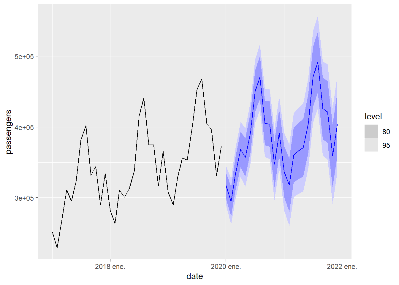
Figure 5.17: 2-year prediction of passenger arrivals in the Canary Islands using the ARIMA model
Double seasonality management
Like the exponential smoothing model, this model is also not designed to directly handle double seasonality. To illustrate a method other than STL decomposition to manage double seasonality, we will present the dynamic harmonic regression method (Dynamic Harmonic Regression) that uses a combination of Fourier series to approximate the seasonality of a time series. A Fourier series of period \(m\) and order \(K\), which we will denote by \(f_{m,K}(t)\), is given by the following combination of trigonometric functions:
\[
f_{m,K}(t)=\sum_{k=0}^K\alpha_k \ cos(\frac{2\pi kt}{m})+\sum_{k=1}^K\beta_k \ sin(\frac{2\pi kt}{m})
\]
Fourier series are a classic way in Mathematical Analysis to approximate periodic functions. The coefficients \(\alpha_k\) and \(\beta_k\) are adapted to fit the periodic function that we want and \(K\) represents the complexity of the approximation, the higher \(K\) is, the better the periodic function will be approximated (but with a higher computational cost), \(m/2\) is the maximum eligible value of \(K\). To eliminate seasonality from the ARIMA model with this method, we apply the ARIMA model without seasonality to the time series \(\tilde{y}_t=y_t-f_{m,K}(t)-f_{m' ,K'}(t)\), where \(m\) and \(m'\) are the periods of the seasonalities involved. The series \(\tilde{y}_t\) corresponds to the series \(y_t\) free of its seasonality. The values of \(K\) and \(K'\) determine the quality of the approximation of \(y_t\) by the Fourier series, the problem is that if \(K\) or \(K'\) are high values, the computational cost to calculate all the parameters can also be high and take a long time to execute. Furthermore, if the original time series has pronounced peaks, as is the case with the ine_comercio_daily series, then the Fourier series has to incorporate many terms (high \(K\) or \(K'\) value) to approximate these peaks. Below is an application of this technique to the ine_daily_trade series:
fit <- ine_daily_trade %>%
   model(
     dhr=ARIMA(value ~ PDQ(0, 0, 0) + pdq(d = 0) + # we use ARIMA without seasonality and without differentiating
                   fourier(period = 7, K = 3) + # we add Fourier series of period m=7 with K=3
                   fourier(period = 365.25, K = 50) # we add Fourier series of period m=365.25 with K=50
              )
   )

  fit %>% #we draw the prediction one year ahead.
   forecast(h = 365) %>%
   autoplot( ine_daily_trade%>%
              filter(date>= as.Date("2022-01-01"))
           )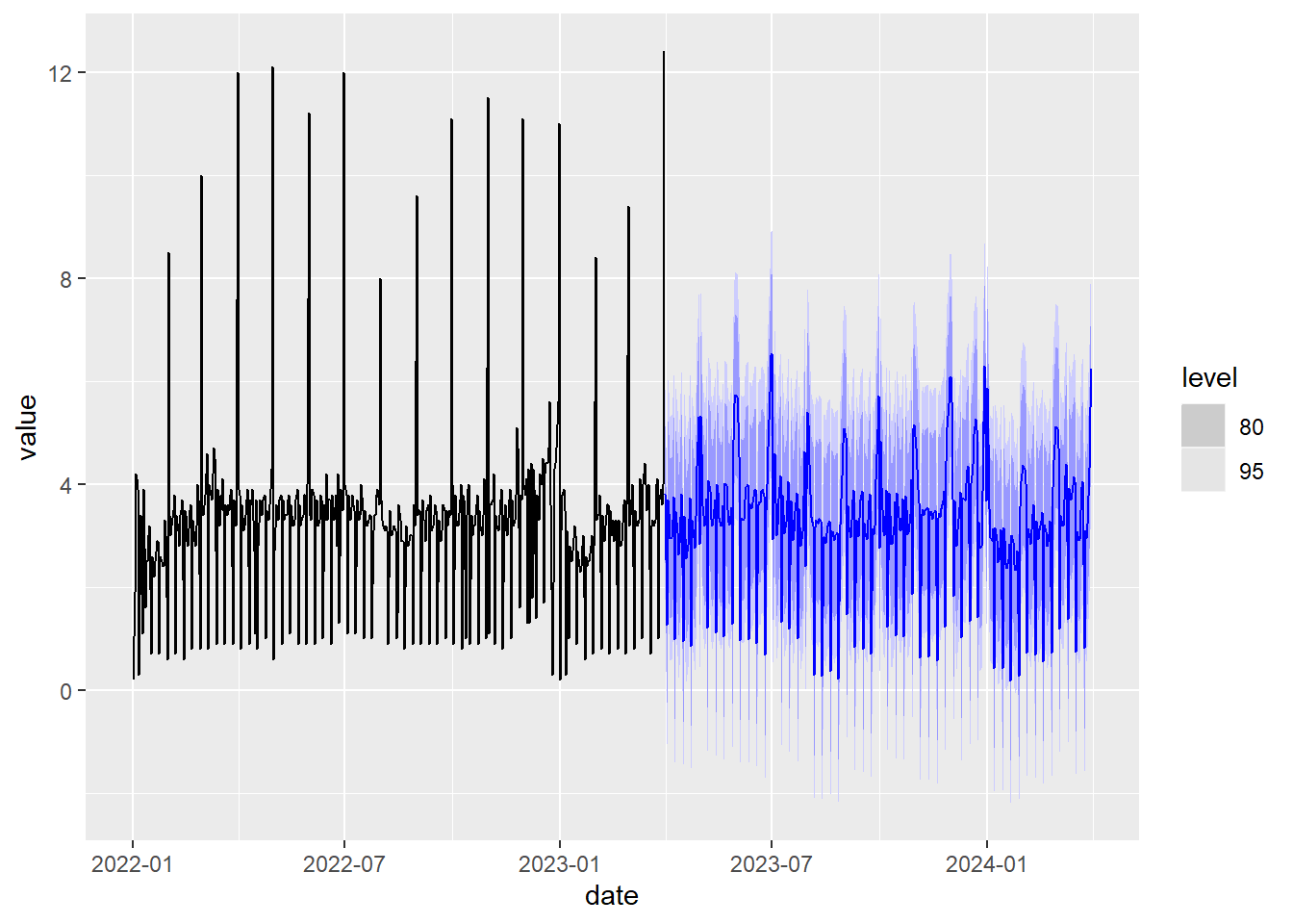
Figure 5.18: Prediction with double seasonality using Fourier series and the ARIMA model
If we run this code, we observe that it takes a long time due to a high value of \(K=50\) and despite this, the peaks of the time series are not predicted well in the future because a higher value of \(K\) would still be needed so that the Fourier series could better approximate these peaks. That is, this technique of managing seasonality with Fourier series works well when the period is small or the time series evolves smoothly and does not have pronounced isolated peaks. The STL decomposition method for handling double seasonality is much faster and handles spikes well without added computational costs.
5.8 Summary prediction models
When applying prediction models, it is important to take into account their working hypotheses. The ETS model assumes that, once seasonality is compensated, the trend of the time series is approximately linear. This linear trend can be gently damped using the damping parameter. The ETS model uses all the past values in the series to make the prediction, but the weight of each value decreases as we go further into the past. The number of numerical parameters of the model grows a lot when there is a seasonality with a high period \(m\), therefore it is not advisable to manage the seasonality within the model for very high \(m\), such as \(m=365\) when we work with a daily data with annual frequency. The ARIMA model assumes that once seasonality is compensated, some derivative of the time series is a “trendless” series, that is, it oscillates around a constant value. The ARIMA model uses only a queue of values towards the past to calculate the prediction, but it has much more freedom than the ETS model to set the elements of the past that participate in the prediction and their weight in the prediction. Furthermore, the number of numerical parameters you need to manage seasonality does not depend on the period \(m\).
As we have seen, simple seasonality can be compensated within the prediction model itself. It can also be compensated outside the model using STL decomposition or Fourier series. These latter techniques allow managing double seasonality, something that cannot be managed within the prediction models studied. The use of Fourier series is not advisable for time series that present strong variations and seasonality with a high \(m\) period.
In this course, to apply prediction models to a time series we use the specialized
Rlibraries and therefore, we will not calculate the configuration and parameters of the models “by hand.” However, it is important to know how to interpret the result obtained to understand what we are doing. For example, the ETS(E,T,S) model has 3 types of options that refer to:- E: Whether the error model is additive or multiplicative.
- T: If the model has a trend and if damping is used. In practice, the usual thing is that the series has some tendency, either to grow or to decrease.
- S: If the model includes seasonality that can be additive or multiplicative.
The interpretation of the parameters of the ARIMA(p,d,q)(P,D,Q)\(_m\) model is:
- \(m\) : the periodicity of seasonality, that is, we expect that every \(m\) days (or temporal units of the series) the series tends to repeat itself. If \(m>1\), this value naturally introduces the \(m\) spaced time series given by \(y_t,y_{t-m},y_{t-2m},y_{t-3m},...\) and the same for the previous series of errors \(\varepsilon_t,\varepsilon _{t-m},\varepsilon _{t-2m},\varepsilon _{t-3m},...\)
- p : size of the queue of the time series values involved in the prediction design.
- P : size of the queue of the \(m\) spaced time series values involved in the prediction design.
- q : size of the queue of values of the error series involved in the prediction design.
- Q : size of the queue of values of the \(m\) spaced error series involved in the prediction design.
- d : order of the derivative of the time series involved in the prediction design.
- D : order of the derivative of the \(m\) spaced time series involved in the prediction design.
The libraries that we use to fit the prediction models provide estimators, such as AIC, AICc and BIC, of the quality of the model fit to the time series for the known data. Although we will not go into the study of these quality estimators here, we will say that the smaller their value, the better the quality of the fit, which allows us to compare the quality of the fit of the models studied. These quality estimators also take into account the number of numerical parameters that are optimized. Using many numerical parameters is considered negative in the quality of the fit due to the aforementioned “overfitting” problem.
The models use the entire series to fit the parameters. If, in the past, the behavior of the series was very different, it may be a good idea to filter the series before making the prediction. It must be taken into account that if there is seasonality, the methods usually require at least 2 complete periods of data, that is, if we have daily data with an annual seasonality (\(m=365.25\)), we need the series to have more than 730 data to manage seasonality.
A prediction without associated confidence intervals is of very little use because without knowing the expected range of fluctuation of the value it is not possible to interpret the expected quality of the result. To illustrate this, let’s imagine predicting a lottery number between 0 and 99999 based on lottery numbers that have been drawn in the past. The expected value of the prediction, which will normally not be far from 50,000, is a completely useless value for predicting the number that will come out today, but without confidence intervals we would not be able to assess the interest and relevance of this prediction. Even if the confidence intervals provided by the models are reasonably small for a short-term prediction, we must be cautious when interpreting them because they assume that the error in the estimate is a normal distribution of constant and decorrelated variance (which we can interpret as the error on one day is independent of the error on the rest of the days). In addition to the fact that, in practice, this is only verified approximately and with a large margin of error, it is assumed that, in the future, the distribution of the daily error is the same, conserving its variance. This is a reasonable hypothesis, at least in the short term, in series that move with stable inertia, such as, for example, a population. However, this hypothesis is not met in series where external events can, in the very short term, completely change the trend of the time series, as in the case, for example, of the stock market quotation, or the price of energy. (note the effect of an event like the war in Ukraine). Even in relatively stable series in the past, such as passenger movements at airports, an event such as the COVID-19 epidemic renders any prediction made in the past useless. That said, with all its associated limitations, making predictions is a fundamental and indispensable element in the decision chain in any company, organization or country.
5.9 Fill gaps in a time series and replace anomalous data.
Sometimes, there are gaps in the time series, that is, data is missing on intermediate dates or there is anomalous data, such as the monthly arrival of travelers at the Canarian airports during the period of the pandemic caused by COVID-19. To study this issue we are going to use data obtained from a query to ISTAC:
istac_airports2 <- read_csv("https://ctim.es/AEDV/data/istac_aeropuertos2.csv")%>%
   as_tibble()%>%
   mutate(month = yearmonth(as.Date(paste0("01/",mes),format="%d/%m/%Y"))) %>%
   as_tsibble(index = month, key = aeropuerto)
istac_airports2 %>%
   autoplot()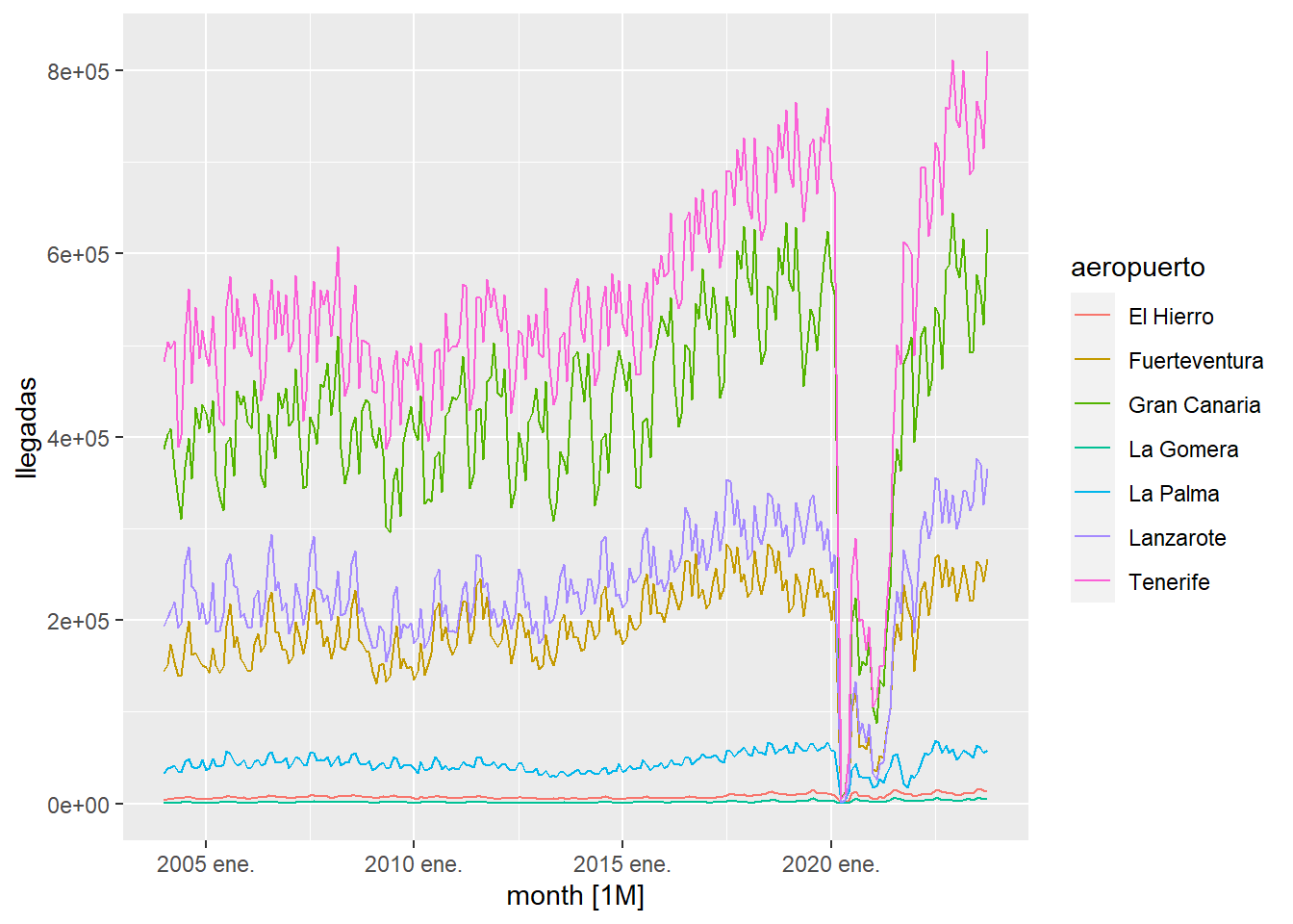
We observe that there is a period of time that is very affected by the pandemic. To study what the time series would have been like if the pandemic had not existed, we will first proceed to eliminate the affected data from the series and then cover it with the fill_gaps function which inserts any missing date and associate NA values to the expected observation:
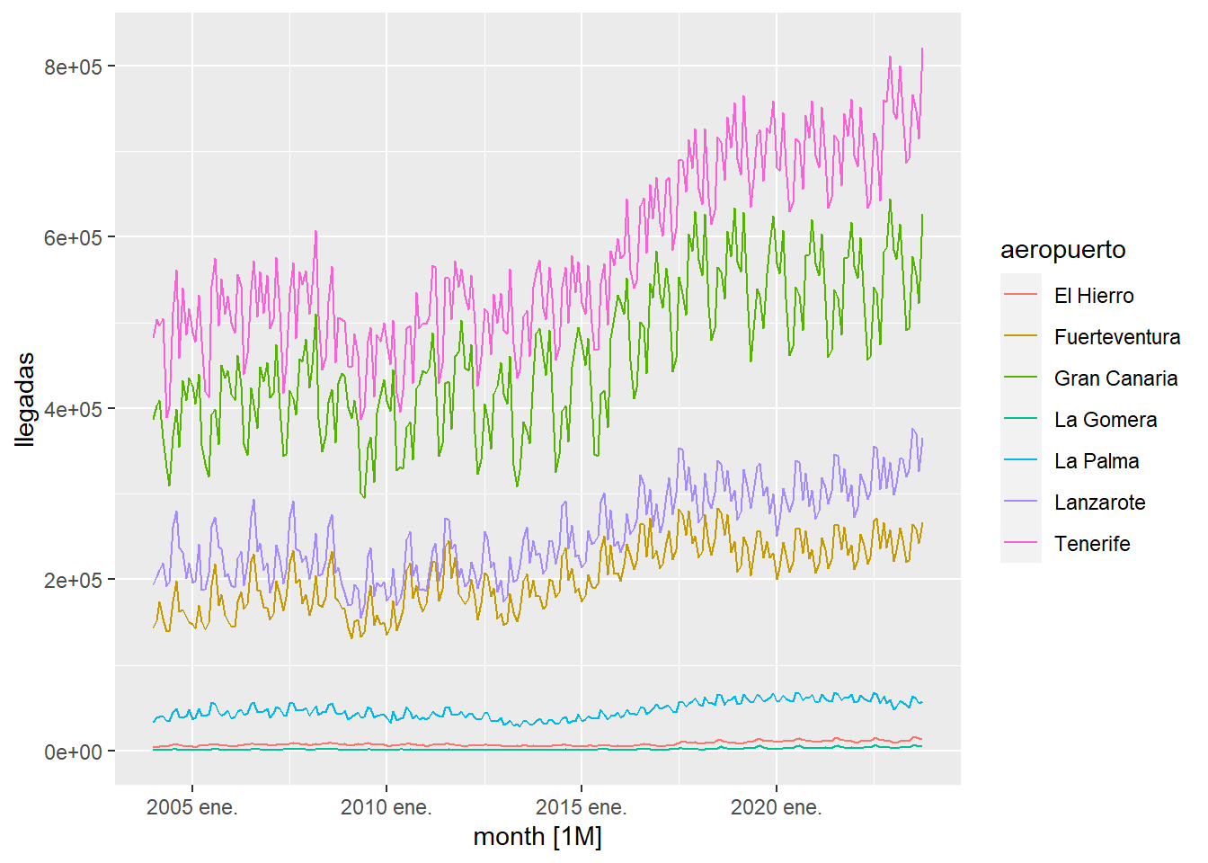
istac_airports2 <- istac_airports2 %>%
   filter(month>=as.Date("2022-06-01") | month<as.Date("2020-02-01") ) %>%
   fill_gaps()

istac_airports2 %>%
   autoplot()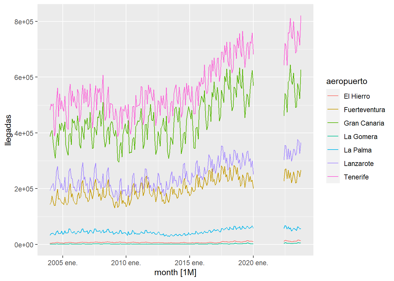
As can be seen in the previous graph, anomalous data no longer appear in the time series. Now what we will do is fill in the gaps created by building an ARIMA model with the existing data and interpolating the missing values with the ARIMA model:
References
[HyAt21] Rob J Hyndman and George Athanasopoulos. Forecasting: Principles and Practice (3rd Ed), OTexts, 2023.
[CCMT90] R. B.,Cleveland, W. S., Cleveland, J. E., McRae, and I. J. Terpenning. STL: A seasonal-trend decomposition procedure based on loess. Journal of Official Statistics, 6(1), 3–33, 1990