Appendix 1. Markdown Syntax
Many of the descriptions of Markdown syntaxes presented here can be obtained directly in the Markdown quick reference section of the RStudio help menu.
Format text with Pandoc
Table format
+---------------+---------------+--------------------+
| A             | B             | C                  |
+===============+===============+====================+
| A0            | B1            | - C10              |
|               |               | - C11              |
+---------------+---------------+--------------------+
| A1            | B2            | - C20              |
|               |               | - C21              |
+---------------+---------------+--------------------+
Compiled result:
| A | B | C |
|---|---|---|
| A0 | B1 |
|
| A1 | B2 |
|
Building a table from a tibble structure
tibble(
   year=c(1985,2000,2015),
   Spain=c(38.734,40.75,46.122),
   France=c(55.38,59.387,64.395),
   Germany=c(77.57,81.896,80.689)) %>%
knitr::kable( caption = "Annual population in millions")| year | Spain | France | Germany |
|---|---|---|---|
| 1985 | 38.734 | 55.380 | 77.570 |
| 2000 | 40.750 | 59.387 | 81.896 |
| 2015 | 46.122 | 64.395 | 80.689 |
Codes in the Markdown file
Chunks
The syntax of the chunks is as follows
Chunk Options
include = FALSEneither the code nor the results appear in the compiled file. R Markdown still runs the code in the chunk and the results can be used by other chunks.echo = FALSEthe code does not appear in the compiled file but the results do.message = FALSEprevents messages generated by the code from appearing in the compiled file.warning = FALSEprevents warnings generated by the code from appearing in the compiled file.cache = TRUEsaves the execution of thechunkand is not executed again unless it is modified. This is interesting to speed up the execution of theKnit.fig.cap = "..."adds a legend to the graphical results.out.width='60%'sets the width of the shape as a percentage of the width of the text area.fig.asp=1.2sets the height/width ratio of the figurefig.align='center'sets the alignment of the figure
Additionally, we can associate a label (label) to each chunk by writing it at the beginning, after ```{r. Let’s look at this with an example of a bar chart figure (in this example the instructions on how to construct the bar chart are not relevant).
```{r chunk-label,fig.cap = "Figure legend",out.width='50%',fig.asp=0.8,fig.align='center',cache=TRUE}
tibble(var=c("A","B","C"),value=1:3) %>%
   ggplot(aes(x=var,y=value,fill=var)) +
     geom_bar(stat = "identity")
```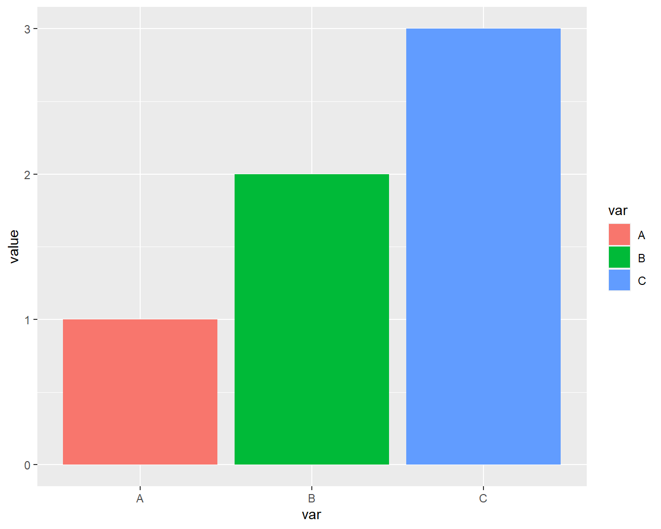
Figure 8.1: Figure legend
If we want to adjust the default options that the chunk will use, we can put an instruction like the following at the beginning of the document, which will ensure that, by default, the chunk code is not included in the text. This is interesting when we want to generate text without R codes.
```
Interactive execution of R code
To debug code errors, it is useful to be able to execute the code line by line. To do this, simply place the cursor over it and press Ctrl-Enter (on Windows and Linux), or Cmd-Enter (on Mac). To execute several lines, we can select them with the mouse and do the same. To execute the entire content of a chunk, simply place the mouse anywhere in the chunk and press Alt-Ctrl-C (on Windows) or Alt-Cmd-Enter (on Mac).