Chapter 5 Chapter 5: Introduction to Generalized Linear Mixed Models

5.1 Introduction to Mixed Models
Sometimes we need to analyze data with a clear hierarchical structure:
- Student level outcomes
- Nested in classroom and schools
- Health outcomes
- Within hospital
- Within county/state
- Over time (how is this different?)
- Political sentiment
- Within states/counties
- Over time
The outcomes may be continuous, binary, counts, ordinal, or nominal. We have a modeling toolkit for different types of outcomes, but we have always assumed that subjects/outcomes were observed independently.
A common design in social and health sciences is the longitudinal study, in which the same questions are asked repeatedly of the same subjects over time. If the outcome were a performance measure, one would not expect large fluctuations over time. If the outcome were a biological characteristic, such as height/weight, it also would tend to be at similar levels over time. This suggests that observations within the same individual are correlated (we sometimes call this autocorrelation). A similar argument applies to students in the same classrooms (their outcomes are correlated, say if taken in pairs), even patients in the same hospital.
5.1.0.1 Exercise 1
Hint is visible here5.1.1 Notation (Nested Case)
- Use \(Y_{ij}\) to denote a two-level clustered/nested outcome, where the first index \(i\) indicates the \(i^{th}\) observation within the \(j^{th}\) cluster, \(i=1,\cdots,n_j\), and the second index \(j\) indicates the \(j^{th}\) cluster, \(j=1,\cdots,J\). The total sample size is \(N=\sum\limits_{j=1}^{J}{{{n}_{j}}}\).
- The levels correspond to the nested nature of the data: level-one is nested in level-two
- The cluster size \(n_j\) can be the same for all \(j\) (balanced design) or different (unbalanced design)
- The cluster size can be small or somewhat large. But in most studies, a fixed number is targeted, if not always obtained.
- In more complex situations, there can be more than two levels. Students/Classroom/School, \(Y_{ijk}\).
- For predictors, the subscripts tell us how much (at what level) that predictor varies.
- Use \(X_{ij}\) to denote covariates whose values vary at both levels.
- Use \(W_j\) to denote covariates whose values only vary at level-two (the cluster, in this case).
5.1.2 Visualization of clustered data
We will simulate data from 10 classrooms in a school. The outcome “Y” is a test score, and the single predictor will be a generic “X” that is used to sort students into classrooms.5
Code
set.seed(2044)
J <- 10  #classrooms
n <- 15  #avg. number of students per classroom
N <- n * J  #total number of records
X <- runif(N)
j <- as.numeric(cut(X, J))  #will assign n-tiles as numbers 1-n
sig.alpha.DGP <- 1.5
sig.eps.DGP <- 0.25
alpha <- rnorm(J, mean = 0, sd = sig.alpha.DGP)  #notice only M values are needed
eps <- rnorm(N, mean = 0, sd = sig.eps.DGP)  #individual level errors
int.coef <- 0
x.coef <- 2
Y <- int.coef + x.coef * X + alpha[j] + eps
meanX <- tapply(X, j, mean)[j]  #for use in plots
meanY <- tapply(Y, j, mean)[j]  #for use in plots
df <- data.frame(id = 1:N, classid = factor(j), X = X, Y = Y, meanX = meanX, meanY = meanY)
ggplot(data = df, aes(x = X, y = Y, group = classid, color = classid)) + geom_point() + geom_segment(aes(x = meanX -
    0.05, y = meanY, xend = meanX + 0.05, yend = meanY))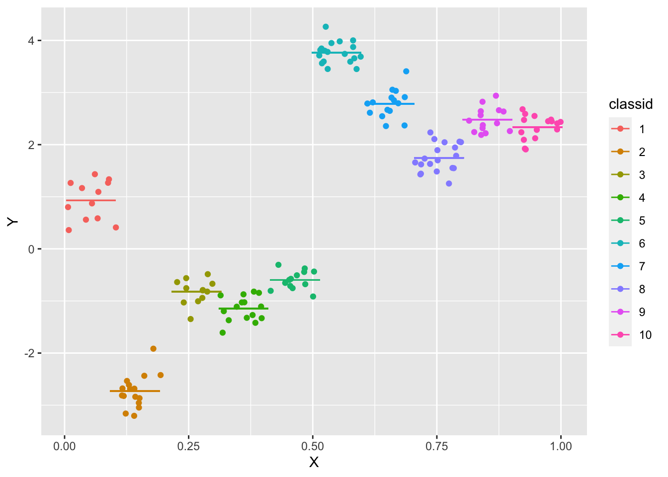
- “Sorting” of students into classrooms by characteristic \(X\) is clear by their perfect separation with respect to \(X\).
- The relationship between \(X\) and \(Y\) is clearly positive, but the impact of \(\alpha_j\) and to some extent \(\varepsilon_{ij}\) (with a small sample in each classroom) weakens its strength.
- The means for each classroom are indicated by line segments of the same color.
- The simple linear regression on these data does not reflect well the relationships used in the DGP:
Code
fit.lm <- lm(Y ~ X, data = df)
summary(fit.lm)
##
## Call:
## lm(formula = Y ~ X, data = df)
##
## Residuals:
## Min 1Q Median 3Q Max
## -2.2928 -1.1736 -0.3979 1.1729 3.2734
##
## Coefficients:
## Estimate Std. Error t value Pr(>|t|)
## (Intercept) -1.6021 0.2588 -6.189 5.64e-09 ***
## X 4.9261 0.4339 11.353 < 2e-16 ***
## ---
## Signif. codes: 0 '***' 0.001 '**' 0.01 '*' 0.05 '.' 0.1 ' ' 1
##
## Residual standard error: 1.508 on 148 degrees of freedom
## Multiple R-squared: 0.4655, Adjusted R-squared: 0.4619
## F-statistic: 128.9 on 1 and 148 DF, p-value: < 2.2e-165.1.3 Problem with clustered data
Observations that belong to the same cluster tend to be correlated due to cluster effect (they belong to the same group).
- For example, students assigned to the classroom with a more effective teacher tend to have higher test scores than students assigned to a different classroom with less effective teacher.
- If some type of controls for these differences between teachers are not included, then the test scores within cluster are correlated, violating a key regression assumption.
- In practice, even if we control for teacher’s effects, students test scores can still be correlated at classroom level due to unobserved effects, which could include peer effects, sorting, etc.
Why do we care about correlation? When cluster level effects are not controlled, the inference will be wrong.
- In a linear model, the standard errors are wrong and typically too small, but the values of the estimated regression coefficients tend to be less affected (unbiased – depending a bit on the design).
- If one runs linear regression on non-normal outcomes, the regression coefficients are biased and standard errors are wrong.
When there are no other cluster level predictors, one can consider using indicator variables to represent each cluster to allow clusters to have different intercepts.
- This may not make sense when there are a lot (>10 ?) of clusters.
- This might be problematic when the data are longitudinal (depending on the inferential goals).
- Use of indicator variables for classroom effects essentially capture the mean level of each class (adjusting for other student covariates); within each class, each student’s test scores varies independently around the class mean.
Including cluster indicators can be an informative way of modeling the clustered data. For example, in a linear regression, \[{{Y}_{ij}}={{X}_{ij}}\beta +{\alpha_{j}}+{{\varepsilon }_{ij}}\] each \(\alpha_j\) in this case is estimated as a coefficient on an indicator \(I\{\mbox{group}=j\}\).
As alluded to above, when there are a lot of clusters, and/or the cluster size is small, we must consider the statistical issues of efficiency and consistency.
- For example, in a household survey, the average cluster (household) size is around 2, we need to estimate thousands of indicator coefficients, each of them is based on an average of 2 observations. Not a good idea!
- Another problem with using cluster indicators is that we cannot simultaneously include cluster level predictors as it induces collinearity! This means that cannot estimate teacher characteristic effects and a unique classroom effect in the same model.
- Modeling the cluster effects via random effects (to be described) is an attractive alternative. Note, however, that the use of random effects is not without some controversies as well.
5.1.4 Random effects
- \(\alpha_j\) is viewed a random variable – we only care about its distribution and the parameters that define it. \(\alpha_j\) is referred to as the random effect.
- \(\alpha_j\sim N(0, \sigma_\alpha^2)\) rather than trying to estimate/predict realized value of each \(\alpha_j\), it suffices to estimate the variance parameter \(\sigma_\alpha^2\) along with the other model parameters (regression coefficients).
- In the rest of the model, the coefficients in the vector \(\beta\) are referred to as fixed effects. In this context, this means that they do not vary over clusters, while the \(\alpha_j\) do.
- A regression model for clustered data that includes both fixed and random effects is called a mixed effect model, but there are other names: multilevel, random effect, random coefficients, hierarchical.
- : When the clusters are represented by indicators variables and the effects \(\alpha_j\) are estimated as coefficients for each cluster, the model is also equivalent to the (econometric) fixed effect model.
5.1.5 Linear Mixed Effects: key terms
Imagine a random effects model for a continuous outcome \(Y_{ij}\) on students in classrooms in a single school.
\[ Y_{ij} = X_{ij}\beta + W_j\delta + \alpha_j + \epsilon_{ij} \] with \(X_{ij}\) student level characteristics, \(W_j\) classroom level characteristics (maybe of the teacher), \(\beta, \delta\) the regression coefficient vectors for the predictors, \(\alpha_j\) a group-(\(j\))-specific random effect, and \(\varepsilon_{ij}\) an individual-specific error term. We usually assume \(\alpha_j\sim N(0, \sigma_\alpha^2)\) and \(\varepsilon_{ij}\sim N(0, \sigma_\varepsilon^2)\), independently of each other, across individuals and in this case classrooms. Net of predictor effects, classroom and student level “error” or variation are assumed independent.
5.1.5.1 Exercise 3
Hint is visible here5.1.6 Random components and their variance
Clearly, \(\alpha_j\) is random, but so is \(\varepsilon_{ij}\). What is interesting about mixed models is that a researcher’s goal is to explain more than one type of variance:
- How much variation in there between student outcomes that is due to being in different classrooms? This is measured by \(\sigma_\alpha^2\).
- Net of classroom differences, how much student-to-student variation remains? This is measured by \(\sigma_\varepsilon^2\).
We call \(\sigma_\alpha^2\) the between group (or cluster) variance, and \(\sigma_\varepsilon^2\) the within group variance, in a manner akin to ANOVA (between vs. within variance). We call the proportion of variance that is attributed between groups (to the total) as the Intraclass Correlation Coefficient (ICC) and define it as follows:
\[ ICC=\frac{\sigma_\alpha^2}{\sigma_\alpha^2+\sigma_\varepsilon^2} \]
- While it is tempting to view this fraction as an \(R^2\), it is not.
- As one explains either within or between variance by including new predictors in the model, the numerator and denominator both change
- In a traditional measure of \(R^2\) in which there is only “within” variance to explain, this does not happen.
5.1.7 Individual- or cluster-specific interpretation
If this were classic regression, we might construct a prediction from our model based on estimates of the parameters and a given covariate pattern. We are predicting the expected value of \(Y_{ij}\) given predictors and the model, so we write:
\[ E(Y_{ij}|X_{ij},W_j,\hat\beta,\hat\delta) = X_{ij}\hat\beta+W_j\hat\delta \] While this works for regression, it is not sufficient for mixed models. We have more information, and that information is contained in the variance components.
- The above describes the “population average” or what might be expected across a sample of clusters within which individuals have exactly those covariate patterns, since \(E(\alpha_j)=0\) for all \(j\).
- But we want to describe our expectations for an individual within a specific cluster. We write this a bit differently.
\[ E(Y_{ij}|X_{ij},W_j,\hat\beta,\hat\delta,\alpha_j) = X_{ij}\hat\beta+W_j\hat\delta + \alpha_j \] We are conditioning on \(\alpha_j\) – this is the cluster-specific perspective.6
You might ask how we know \(\alpha_j\)? We don’t. This discussion is based on the idea that if we were to know the value \(\alpha_j\), we would include it in our prediction for anyone in cluster \(j\). There is a common approach to “predicting” the value of \(\alpha_j\) a posteriori (after fitting the model and estimating the parameters). This prediction is called the BLUP and is defined as:
\[ \hat\alpha_j=E(\alpha_j|X_{ij},W_j,\hat\beta,\hat\delta,\hat\sigma_\alpha^2,\hat\sigma_\varepsilon^2, Y_{\cdot j}) \]
- You might be surprised by the inclusion of variance component estimates. They, along with the ICC serve to calibrate the value of \(\hat\alpha_j\) using information from the observations within that group.
- You might be more surprised by the inclusion of \(Y_{\cdot j}\), which stands for all observations in group \(j\). One way to understand its inclusion is that one must identify how much above or below 0 the deviation of the entire group is from the population average.
5.1.8 Model Estimation
In the normal error and random effect case, we can explicitly write down the DGP for the outcome vector \(\vec{Y}=\{Y_{ij}\}_{ij}\), where \(i\) ranges over the indices \(1,\ldots,n_j\) for each cluster \(j\), and \(j\) follows the ordering \(1,\ldots,J\) for \(J\) groups.
We drop the cluster-constant predictor \(W_j\) for simplicity. Given
\[ Y_{ij} = X_{ij}\beta + \alpha_j + \epsilon_{ij} \]
with \(\alpha_j\sim N(0, \sigma_\alpha^2)\) and \(\varepsilon_{ij}\sim N(0, \sigma_\varepsilon^2)\) independent across and within groups. \[ \vec{Y}\sim N(X\beta,\Sigma)\ \ \mbox{ with } \Sigma=\sigma_\alpha^2ZZ'+\sigma_\varepsilon^2I_N \] \(X\) is a matrix, with each row \(X_{ij}\), \(Z\) is also a matrix, with each row \(Z_{ij}=Z_j\) duplicating the random effects design across all individuals in group \(j\), and \(I_N\) is an \(N\times N\) identity matrix.
- In this discussion, with a single random intercept, \(Z\) is the design associated with cluster membership, so for an example with 3 groups of size 3, it could look like this:
Code
clust <- factor(rep(1:3, each = 3))
mat <- model.matrix(~-1 + clust)
mat
## clust1 clust2 clust3
## 1 1 0 0
## 2 1 0 0
## 3 1 0 0
## 4 0 1 0
## 5 0 1 0
## 6 0 1 0
## 7 0 0 1
## 8 0 0 1
## 9 0 0 1
## attr(,"assign")
## [1] 1 1 1
## attr(,"contrasts")
## attr(,"contrasts")$clust
## [1] "contr.treatment"In this simplest case of a random intercept model, the term \(ZZ'\) creates a block diagonal structure, like this:
Code
mat %*% t(mat)## 1 2 3 4 5 6 7 8 9
## 1 1 1 1 0 0 0 0 0 0
## 2 1 1 1 0 0 0 0 0 0
## 3 1 1 1 0 0 0 0 0 0
## 4 0 0 0 1 1 1 0 0 0
## 5 0 0 0 1 1 1 0 0 0
## 6 0 0 0 1 1 1 0 0 0
## 7 0 0 0 0 0 0 1 1 1
## 8 0 0 0 0 0 0 1 1 1
## 9 0 0 0 0 0 0 1 1 1Putting the pieces together, we can see how the covariance matrix \(\Sigma=\sigma_\alpha^2ZZ'+\sigma_\varepsilon^2I_N\) has block diagonal components that look like this:
\[ \begin{pmatrix} \sigma_\alpha^2+\sigma_\varepsilon^2 & \sigma_\alpha^2 & \sigma_\alpha^2 \\ \sigma_\alpha^2 & \sigma_\alpha^2+\sigma_\varepsilon^2 & \sigma_\alpha^2 \\ \sigma_\alpha^2 & \sigma_\alpha^2 & \sigma_\alpha^2+\sigma_\varepsilon^2 \end{pmatrix} \]
- This structure is called compound symmetry in the RMANOVA and mixed models literature, and exchangeability in other contexts, as the implied correlation within groups is always the same (individuals are exchangeable within group with respect to covariance structure).
- The ICC for this model is given by \(\frac{\sigma_\alpha^2}{\sigma_\alpha^2+\sigma_\varepsilon^2}\) and this is also the correlation between pairs of observations within the same cluster, net of predictor effects.
5.1.9 Model Fit: Simulated Data
Returning to our simulated data, how would we model it correctly, and what changes would we observe in the model estimates?
- The
Rpackagelme4or better,lmerTestcontains a functionlmerthat is the mixed effects extension oflmfor linear models and normal errors. There is aglmerfunction for generalized linear mixed models as well. - The syntax for the formula portion of the model can be quite complex, but for simple random intercept models, it involves merely adding
+(1|id)whereidis the unique cluster or group identifier in your data. lmermodels are fit using the method of maximum likelihood, e.g., based on an EM algorithm.
Code
fit <- lmerTest::lmer(Y ~ X + (1 | classid), data = df)
summary(fit)
## Linear mixed model fit by REML. t-tests use Satterthwaite's method ['lmerModLmerTest']
## Formula: Y ~ X + (1 | classid)
## Data: df
##
## REML criterion at convergence: 78.1
##
## Scaled residuals:
## Min 1Q Median 3Q Max
## -2.47289 -0.64723 0.04191 0.60643 2.82914
##
## Random effects:
## Groups Name Variance Std.Dev.
## classid (Intercept) 2.93527 1.713
## Residual 0.06553 0.256
## Number of obs: 150, groups: classid, 10
##
## Fixed effects:
## Estimate Std. Error df t value Pr(>|t|)
## (Intercept) -0.2971 0.6562 15.8252 -0.453 0.6569
## X 2.3219 0.7322 128.5225 3.171 0.0019 **
## ---
## Signif. codes: 0 '***' 0.001 '**' 0.01 '*' 0.05 '.' 0.1 ' ' 1
##
## Correlation of Fixed Effects:
## (Intr)
## X -0.563Code
fe <- lme4::fixef(fit)
fe.tbl <- summary(fit)$coef
sig.alpha <- attr(lme4::VarCorr(fit)["classid"]$classid, "stddev")
sig.eps <- fit@sigma
alphas <- lme4::ranef(fit)
5.1.10 Interpreting the results
Fixed effects:
- The fixed effect estimated for the intercept of -0.3 with p-value 0.66; the DGP value is 0.
- The fixed effect estimated for the slope on \(X\) of 2.32 with p-value 0; the DGP value is 2.
- The confidence interval surrounding our estimate of the \(X\) effect is (0.89, 3.83), which easily contains the true value.
Variance components:
- The estimated standard deviation for the random effects is \(\hat\sigma_\alpha=\) 1.71; the DGP value is 1.5.
- The estimated standard deviation for the individual-level error is \(\hat\sigma_\varepsilon=\) 0.26; the DGP value is 0.25.
- There are no standard errors associated with these variance components (and if they were reported, they would not be used in the manner to which you are accustomed).
- Estimates (really predictions, in this context) of each \(\alpha_j\) are labeled “BLUP” and given in the table below, with the DGP generated values as well.
Code
alphas <- lme4::ranef(fit)
tbl <- data.frame(j = 1:J, BLUP = alphas$classid$`(Intercept)`, DGP = alpha)
knitr::kable(tbl, digits = 2)| j | BLUP | DGP |
|---|---|---|
| 1 | 1.10 | 0.83 |
| 2 | -2.76 | -2.95 |
| 3 | -1.14 | -1.32 |
| 4 | -1.69 | -1.91 |
| 5 | -1.38 | -1.34 |
| 6 | 2.79 | 2.60 |
| 7 | 1.56 | 1.51 |
| 8 | 0.29 | 0.27 |
| 9 | 0.80 | 0.80 |
| 10 | 0.42 | 0.48 |
Residuals:
- Since we can predict these BLUPs for the \(\hat\alpha_j\) after estimating the model, this implies there are two types of residuals:
- Group level: the \(\hat\alpha_j\)
- Individual level: \(\hat\varepsilon_{ij} = Y_{ij} - (X_{ij}\hat\beta+\hat\alpha_j)\). Note that in more complex random effects models, we could have more random effects (often called random slopes depending on the context).
- The BLUPs are predicted values of \(\alpha_j\) after fitting the model, and the residuals are estimates of \(\varepsilon_{ij}\) after fitting the model and predicting \(\alpha_j\).
5.1.11 What happens if we forget to control for random effects?
We did this earlier, but it is useful to summarize the results and contrast them to the above mixed model.
Code
summary(fit.lm)##
## Call:
## lm(formula = Y ~ X, data = df)
##
## Residuals:
## Min 1Q Median 3Q Max
## -2.2928 -1.1736 -0.3979 1.1729 3.2734
##
## Coefficients:
## Estimate Std. Error t value Pr(>|t|)
## (Intercept) -1.6021 0.2588 -6.189 5.64e-09 ***
## X 4.9261 0.4339 11.353 < 2e-16 ***
## ---
## Signif. codes: 0 '***' 0.001 '**' 0.01 '*' 0.05 '.' 0.1 ' ' 1
##
## Residual standard error: 1.508 on 148 degrees of freedom
## Multiple R-squared: 0.4655, Adjusted R-squared: 0.4619
## F-statistic: 128.9 on 1 and 148 DF, p-value: < 2.2e-16Code
confint(fit.lm)## 2.5 % 97.5 %
## (Intercept) -2.113637 -1.090602
## X 4.068648 5.783536- The parameter estimates are pretty far from the known values (from the DGP).
- We are overly confident in those estimates – s.e. are too small, so the confidence intervals do not contain the truth.
- The residual standard error should be the square root of the sum of the between and within variances in the mixed model.
- The “bias” in the regression parameters should diminish as the number of groups and size of each group grows.
5.2 Generalized Linear Mixed Effect Models (GLMMs)
GLMMs are extensions of Linear Mixed Models (or multilevel models) that allow us to examine outcomes that are not normally distributed, such as binary and count data, when the observations are clustered under some pre-existing grouping structure.
- When we generalized the linear model to the generalized linear model (GLM) such as logistic regression, probit regression and Poisson regression, we did so by introducing a link function for the mean of the distribution as follows: \[ g(E(Y|X))=\eta=X\beta \]
- We also established some common link functions, which we reproduce here:
- For GLMM, to accommodate random effects, all we need to do is to expand the equation for the conditional mean of the process. We do this for the simplest case of random intercept: \[ g(E(Y|X,\alpha))=\eta+\alpha=X\beta + \alpha \]
\[ \alpha\sim N(0,\sigma_\alpha^2) \]
- \(g(\cdot)\) will depend on the type of outcome.
- We leave \(\alpha\) in the expression for the mean, \(\eta\), as it plays a different role in the likelihood and we will need to be able to separate it out.
- We can estimate the parameters of interest, \(\beta\), \(\sigma_\alpha^2\), using maximum likelihood estimation related methods in the GLMM models (it is actually very complicated!)
Take logistic regression as an example: \[ \log\frac{p_{ij}}{1-p_{ij}}=X_{ij}\beta+\alpha_j \Rightarrow \ p_{ij}=\frac{e^{X_{ij}\beta+\alpha_j}}{1+e^{X_{ij}\beta+\alpha_j}} \] Now we can write down the marginalized log-likelihood function and maximize it over the set of parameters of interest. \[ L(\beta ,\sigma_\alpha^2|Y,X)=\prod\limits_{j=1}^{J}{\int{\prod\limits_{i=1}^{n_j}p_{ij}^{Y_{ij}}(1-p_{ij})^{1-Y_{ij}}f_\alpha(u)du} } \] which give our assumptions, translates to: \[ L(\beta ,\sigma_\alpha^2|Y,X)=\prod\limits_{j=1}^{J}{\int{\prod\limits_{i=1}^{n_j} \left(\frac{e^{X_{ij}\beta+u}}{1+e^{X_{ij}\beta+u}}\right) ^{Y_{ij}}\left(\frac{1}{1+e^{X_{ij}\beta+u}}\right) ^{1-Y_{ij}}\frac{1}{\sqrt{2\pi}\sigma_\alpha}e^{-\frac{u^2}{2\sigma_\alpha^2}}du} } \]
- Closed forms (solving the integral) for the GLMM type of likelihood are rare, so numerical integration methods may be involved.
- In another approach, some iterative process is used: think of it as swapping between estimates for the fixed effects conditional on the random effects and vice versa.
- Bayesian estimation (and inference) techniques are well-suited to this multilevel distributional framework.
5.2.1 Longitudinal Data
We can “reuse” the framework for nested data in the longitudinal case.
- Think of subjects as the grouping factor and occasions of measurement as nested within them: \(Y_{ti}\) is the outcome for person \(i\) at occasion \(t\).
- The most important addition in a longitudinal data model is the inclusion of time. It could be measured age, calendar year, or even occasion number. For now, we will call it \(TIME_{ti}\), which is the time variable at occasion \(t\) for subject \(i\).
- Within-subject correlation must be controlled. The simplest model is again, random intercepts, which implicitly posits that individuals differ from each other in level only.
- More complex longitudinal data models allow individuals to have different trajectories over time. These growth curve models are the subject of another course.
5.2.2 Simulated data
We will simulate normal outcome data first, to ground the concepts.
Code
set.seed(2044)
I <- 10  #subjects
n <- 10  #number of time points per subject
N <- n * I  #total number of records
X <- runif(N)  #observation times - uniform across (0,1)
i <- rep(1:I, each = n)
sig.alpha.DGP <- 1.5
sig.eps.DGP <- 0.25
alpha <- rnorm(I, mean = 0, sd = sig.alpha.DGP)  #notice only M values are needed
eps <- rnorm(N, mean = 0, sd = sig.eps.DGP)  #individual level errors
int.coef <- 0
x.coef <- 2
Y <- int.coef + x.coef * X + alpha[i] + eps
df <- data.frame(id = 1:N, subjID = factor(i), X = X, Y = Y)
ggplot(data = df, aes(x = X, y = Y, group = subjID, color = subjID)) + geom_point() + geom_smooth(method = "lm",
    se = F)
## `geom_smooth()` using formula = 'y ~ x'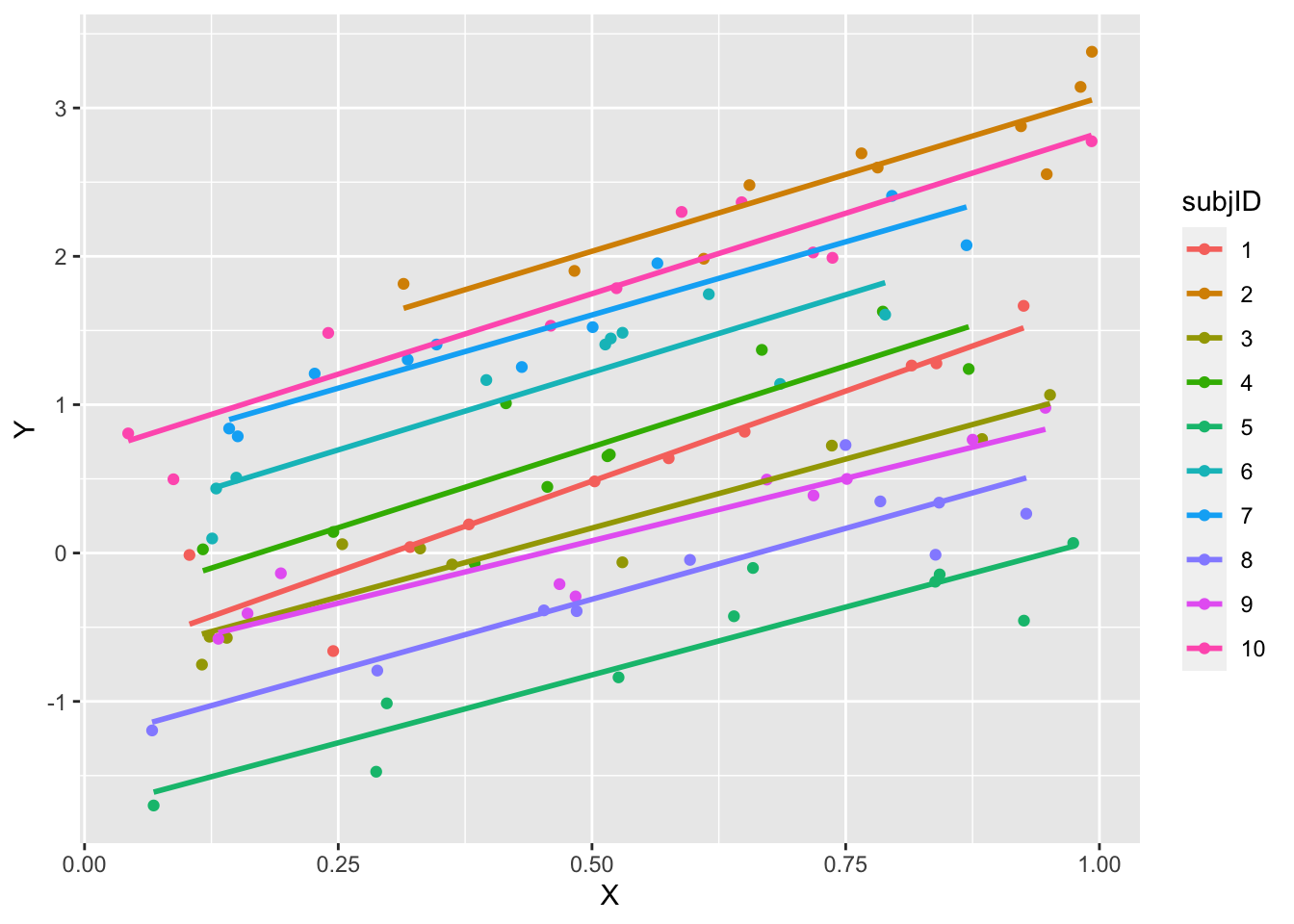
- The lines are approximately parallel, as constructed according to the DGP
5.2.2.1 Exercise 4
Exercise: Discuss and explain: why aren’t the lines exactly parallel?
Each subject is observed the same number of times, but at different time points
We relied on the outcome being continuous; what if it were binary? How could we summarize the data in a visualization?
Hint is visible here
5.2.3 Fitted longitudinal data model
Code
fit <- lmerTest::lmer(Y ~ X + (1 | subjID), data = df)
summary(fit)
## Linear mixed model fit by REML. t-tests use Satterthwaite's method ['lmerModLmerTest']
## Formula: Y ~ X + (1 | subjID)
## Data: df
##
## REML criterion at convergence: 50.9
##
## Scaled residuals:
## Min 1Q Median 3Q Max
## -2.70794 -0.48847 -0.04111 0.57354 2.25463
##
## Random effects:
## Groups Name Variance Std.Dev.
## subjID (Intercept) 0.89802 0.9476
## Residual 0.05793 0.2407
## Number of obs: 100, groups: subjID, 10
##
## Fixed effects:
## Estimate Std. Error df t value Pr(>|t|)
## (Intercept) -0.30734 0.30467 9.49166 -1.009 0.338
## X 1.99899 0.09229 89.14039 21.660 <2e-16 ***
## ---
## Signif. codes: 0 '***' 0.001 '**' 0.01 '*' 0.05 '.' 0.1 ' ' 1
##
## Correlation of Fixed Effects:
## (Intr)
## X -0.162The parameters used in this model were extremely similar to those used in the classroom simulated data example.
5.2.4 Binary Outcome example
Which treatment is best for toenail infection?
- This is a clinical trial data, 378 patients were randomly assigned to two oral antifungal treatments, and are evaluated at seven visits, roughly at weeks 0, 4, 8, 12, 24, 36 and 48.
- One outcome of interest is onycholysis–the degree of separation of the nail plate from the nail bed: 1=moderate or severe; 0 = none or mild.
- We fail to collect any data on the outcomes for 84 of 378 patients. For the rest of the 294 patients, the outcome of at least one visit is measured.
- These data are unbalanced: patients are not observed at equal time intervals (although an attempt was made); and incomplete: many visits are missing at the patient-visit level.
We retrieve the toenail dataset in R with data("toenail", package = "HSAUR2"). It contains these variables:
patient:       patient id
outcome:       onycolysis: 1=moderate or severe; 0 = none or mild
treatment:     0=treatment A; 1=treatment B
visit:         visit number (1,2,...,7)
time:          exact timing of visit (fractions of months)
Translating this to our notation:
- \(i\) is the patient id
- \(t\) is the visit number
- \(Y_{ti}\) is outcome, and it’s binary
- \(W_{i}\) is the treatment arm, which does not change over time (\(t\))
- \(TIME_{ti}\) in these data is collected in
time(which could also be thought of as an \(X_{ti}\) due to the way it varies by person and occasion)
5.2.5 Naive Analysis
- On average, which treatment group has lower infection rate (implies more effective)?
- How should we compare the outcomes based on randomized trial?
- Simply compare the overall infection rates between treatment A and treatment B
# Install HSAUR2 package
install.packages("HSAUR2")

# import data "toenail"
data("toenail", package = "HSAUR2")
Code
data("toenail", package = "HSAUR2")
prettyR::xtab(~treatment + outcome, data = toenail, chisq = T)
## Crosstabulation of treatment by outcome
## outcome
## treatme none or moderate
## itracona 723 214 937
## 77.16 22.84 -
## 48.20 52.45 49.11
##
## terbinaf 777 194 971
## 80.02 19.98 -
## 51.80 47.55 50.89
##
## 1500 408 1908
## 78.62 21.38 100.00
## X2[1]=2.152, p=0.142358
##
## odds ratio = 0.84
## phi = -0.035- The Odds Ratio is 0.84 (p=0.128)
- Odds of moderate vs. none are 0.84 lower in Treatment A vs. B.
- What are the issues with this comparison?
- Individuals contribute different numbers of outcomes at various numbers of visits at various times, but they are all weighted equally.
- Disease progresses as a function of time
- We could take last observation from each person and redo; this would partially fix some of the above issues.
Code
toenailLast <- toenail %>%
    group_by(patientID) %>%
    arrange(patientID, time) %>%
    filter(row_number() == n())
prettyR::xtab(~treatment + outcome, data = as.data.frame(toenailLast), chisq = T)
## Crosstabulation of treatment by outcome
## outcome
## treatme none or moderate
## itracona 129 17 146
## 88.36 11.64 -
## 47.96 68.00 49.66
##
## terbinaf 140 8 148
## 94.59 5.41 -
## 52.04 32.00 50.34
##
## 269 25 294
## 91.5 8.5 100.0
## X2[1]=2.918, p=0.08758135
##
## odds ratio = 0.43
## phi = -0.112While this is probably a better analysis, it still suffers from different endpoints varying by subject.
- Given the longitudinal design, we should use statistical models that:
- Capture the autocorrelation structure in some manner
- Allow for varying number of observations per subject (imbalance, incompleteness)
- Reflect the underlying DGP (limited dependent nature) for the specific type of outcome.
- GLMMs for binary longitudinal data are appropriate in this context.
- First, we attempt to “explore” graphically these data by taking a sample and plotting the “curve” over time.
- This reflects the underlying structure more accurately. Or does it?
Code
set.seed(2044)
samp <- sample(unique(toenail$patientID), 15)
toesamp <- toenail %>%
    filter(patientID %in% samp)
ggplot(data = toesamp, aes(x = time, y = outcome, group = patientID, color = patientID)) + geom_jitter(width = 0.1,
    height = 0.05) + stat_smooth(span = 0.4, se = F)
## `geom_smooth()` using method = 'loess' and formula = 'y ~ x'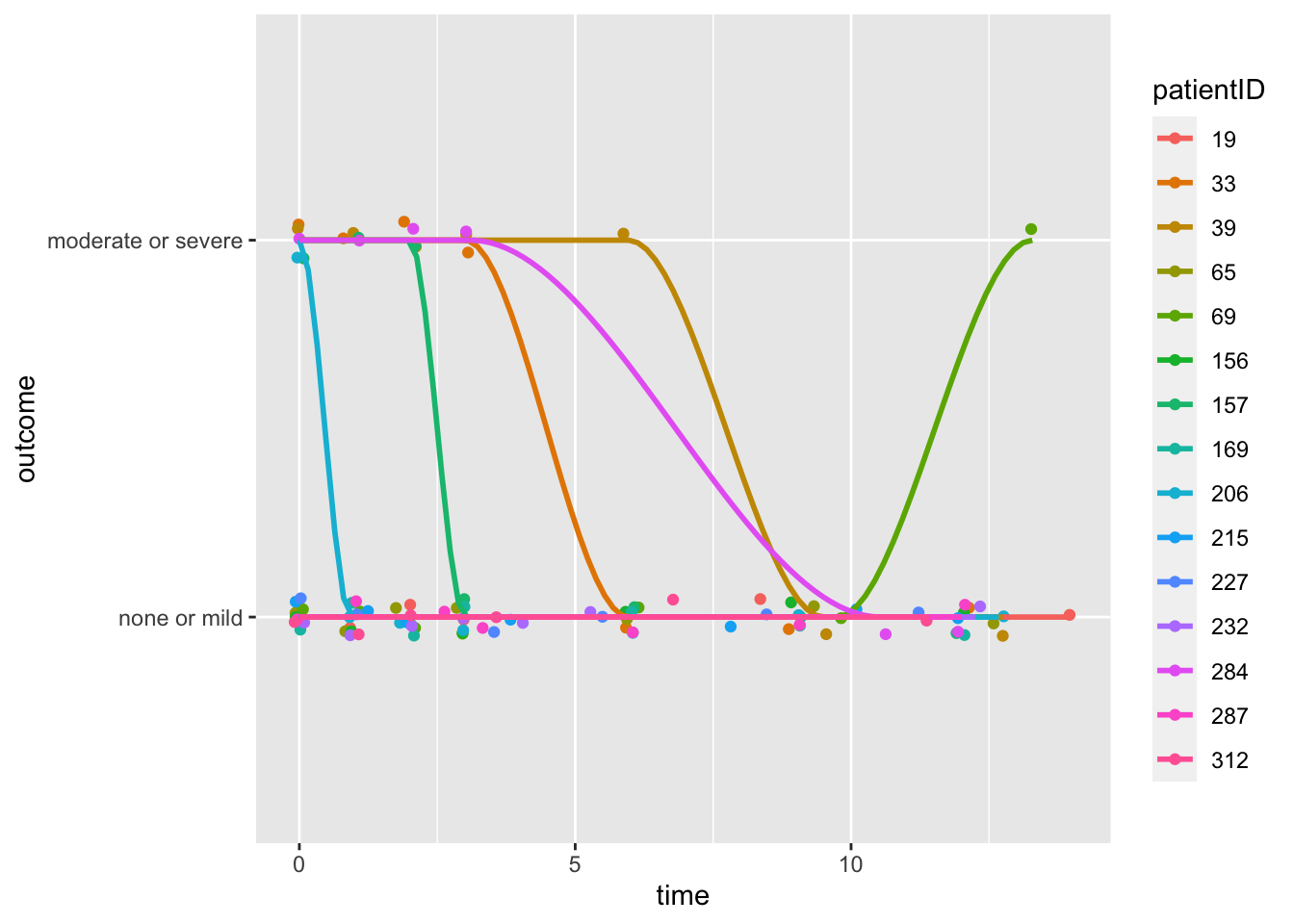
5.2.5.1 Exercise 5
Exercise: What does the plot tell us about individual differences? Why does it appear that only a few curves are drawn?
This visualization of a few subjects is somewhat useful, but it does not provide us with any insight about treatment effectiveness.
To examine treatment differences, we must pool across individuals, which is less true to the data structure, but still somewhat informative.
Hint is visible here
Code
ggplot(data = toenail, aes(x = time, y = outcome, group = treatment, color = treatment)) + geom_jitter(width = 0.1,
    height = 0.05) + stat_smooth(method = "gam", formula = y ~ s(x), se = F)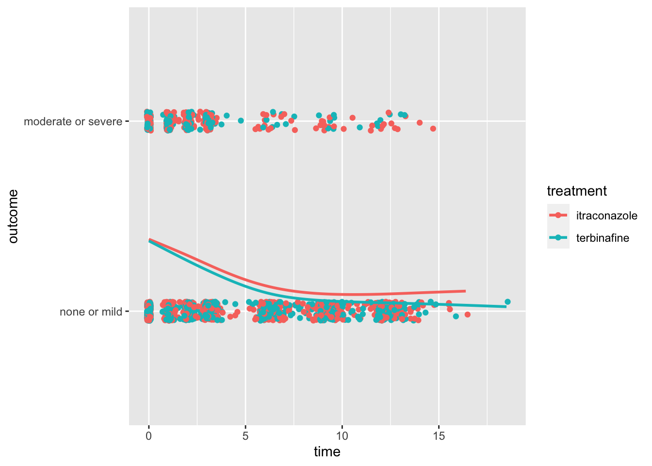
- Apparently, terbinafine, treatment B, is a bit more effective, on average
- Its smoothed curve, which is approximately a probability of moderate or severe symptoms (as compared to mild or none) is lower on the plot, over time.
5.2.5.2 Exercise 6
Hint is visible hereA model that allows for individual differences as well as captures predictor average effects allows us to move beyond a suggestive plot to be able to potentially draw conclusions.
Code
fit.glmer <- lme4::glmer(outcome ~ time + treatment + (1 | patientID), family = binomial, data = toenail)
summary(fit.glmer)
## Generalized linear mixed model fit by maximum likelihood (Laplace Approximation) ['glmerMod']
## Family: binomial ( logit )
## Formula: outcome ~ time + treatment + (1 | patientID)
## Data: toenail
##
## AIC BIC logLik deviance df.resid
## 1267.6 1289.9 -629.8 1259.6 1904
##
## Scaled residuals:
## Min 1Q Median 3Q Max
## -3.7315 -0.1399 -0.0740 -0.0088 30.1542
##
## Random effects:
## Groups Name Variance Std.Dev.
## patientID (Intercept) 20.73 4.553
## Number of obs: 1908, groups: patientID, 294
##
## Fixed effects:
## Estimate Std. Error z value Pr(>|z|)
## (Intercept) -2.31940 0.74733 -3.104 0.00191 **
## time -0.46094 0.03963 -11.632 < 2e-16 ***
## treatmentterbinafine -0.68556 0.65901 -1.040 0.29821
## ---
## Signif. codes: 0 '***' 0.001 '**' 0.01 '*' 0.05 '.' 0.1 ' ' 1
##
## Correlation of Fixed Effects:
## (Intr) time
## time 0.280
## trtmnttrbnf -0.364 0.081- Non-significant treatment effect?
- Model misspecification?
- Does the model reflect the relationship captured in the visualization?
Code
fit2.glmer <- lme4::glmer(outcome ~ time * treatment + (1 | patientID), family = binomial, data = toenail)
summary(fit2.glmer)
## Generalized linear mixed model fit by maximum likelihood (Laplace Approximation) ['glmerMod']
## Family: binomial ( logit )
## Formula: outcome ~ time * treatment + (1 | patientID)
## Data: toenail
##
## AIC BIC logLik deviance df.resid
## 1265.6 1293.4 -627.8 1255.6 1903
##
## Scaled residuals:
## Min 1Q Median 3Q Max
## -3.290 -0.149 -0.071 -0.006 47.215
##
## Random effects:
## Groups Name Variance Std.Dev.
## patientID (Intercept) 20.76 4.557
## Number of obs: 1908, groups: patientID, 294
##
## Fixed effects:
## Estimate Std. Error z value Pr(>|z|)
## (Intercept) -2.50987 0.76392 -3.286 0.00102 **
## time -0.39973 0.04679 -8.543 < 2e-16 ***
## treatmentterbinafine -0.30483 0.68707 -0.444 0.65729
## time:treatmentterbinafine -0.13714 0.06949 -1.973 0.04846 *
## ---
## Signif. codes: 0 '***' 0.001 '**' 0.01 '*' 0.05 '.' 0.1 ' ' 1
##
## Correlation of Fixed Effects:
## (Intr) time trtmnt
## time 0.130
## trtmnttrbnf -0.374 0.220
## tm:trtmnttr 0.181 -0.541 -0.265- Significant treatment by time interaction. What does it mean?
- What about other functional forms? Quadratic change over time, e.g.?
- The logistic transform captures non-linearity implicitly.
Code
fit3.glmer <- lme4::glmer(outcome ~ poly(time, 2) + treatment + (1 | patientID), family = binomial, data = toenail)
summary(fit3.glmer)
## Generalized linear mixed model fit by maximum likelihood (Laplace Approximation) ['glmerMod']
## Family: binomial ( logit )
## Formula: outcome ~ poly(time, 2) + treatment + (1 | patientID)
## Data: toenail
##
## AIC BIC logLik deviance df.resid
## 1249.0 1276.8 -619.5 1239.0 1903
##
## Scaled residuals:
## Min 1Q Median 3Q Max
## -5.2189 -0.1496 -0.0570 -0.0110 16.2783
##
## Random effects:
## Groups Name Variance Std.Dev.
## patientID (Intercept) 23.41 4.839
## Number of obs: 1908, groups: patientID, 294
##
## Fixed effects:
## Estimate Std. Error z value Pr(>|z|)
## (Intercept) -4.7781 1.0024 -4.767 1.87e-06 ***
## poly(time, 2)1 -80.1241 6.9783 -11.482 < 2e-16 ***
## poly(time, 2)2 22.5316 4.9283 4.572 4.83e-06 ***
## treatmentterbinafine -0.7096 0.7017 -1.011 0.312
## ---
## Signif. codes: 0 '***' 0.001 '**' 0.01 '*' 0.05 '.' 0.1 ' ' 1
##
## Correlation of Fixed Effects:
## (Intr) p(,2)1 p(,2)2
## poly(tm,2)1 0.498
## poly(tm,2)2 -0.225 -0.049
## trtmnttrbnf -0.265 0.078 -0.0335.2.6 What if we had neglected the repeated measures design?
In the toenail data:
Code
fit2.glm <- glm(outcome ~ time * treatment, family = binomial, data = toenail)
summary(fit2.glm)
##
## Call:
## glm(formula = outcome ~ time * treatment, family = binomial,
## data = toenail)
##
## Deviance Residuals:
## Min 1Q Median 3Q Max
## -0.9519 -0.7892 -0.5080 -0.2532 2.7339
##
## Coefficients:
## Estimate Std. Error z value Pr(>|z|)
## (Intercept) -0.5566273 0.1089628 -5.108 3.25e-07 ***
## time -0.1703078 0.0236199 -7.210 5.58e-13 ***
## treatmentterbinafine -0.0005817 0.1561463 -0.004 0.9970
## time:treatmentterbinafine -0.0672216 0.0375235 -1.791 0.0732 .
## ---
## Signif. codes: 0 '***' 0.001 '**' 0.01 '*' 0.05 '.' 0.1 ' ' 1
##
## (Dispersion parameter for binomial family taken to be 1)
##
## Null deviance: 1980.5 on 1907 degrees of freedom
## Residual deviance: 1816.0 on 1904 degrees of freedom
## AIC: 1824
##
## Number of Fisher Scoring iterations: 5- s.e. are smaller, but coefficients are biased in model that fails to control for autocorrelation, and it does not lead to same conclusions!
- In general, the fixed effects (coefficients) are attenuated if the clustering effect is not properly controlled and modeled.
5.2.7 ICC
- Understanding (ICC) in Hierarchical Logistic Regression
- In hierarchical linear regression the intra-class correlation is \[ ICC=\frac{\sigma_\alpha^2}{\sigma_\alpha^2+\sigma_\varepsilon^2} \]
- While we can estimate \(\sigma_\alpha^2\) in a GLMM, in hierarchical logistic regression, the individual level error term is not modeled explicitly.
- To establish the notion of error in this context, we borrow the latent variable construct \(Y_{ti}^{*}\) as in probit regression: \[ Y_{ti}^{*}=X_{ti}\beta +\alpha_i+\varepsilon_{ti} \]
- In probit, \(\varepsilon\) is assumed to have standard normal distribution, with variance 1.
- From these choices (restrictions), we can identify the model, and set \(Y_{ti}=1\) when \(Y_{ti}^{*}>0\).
- Analogously, we can assume \(\varepsilon\) follows a logistic distribution, with mean 0 and scale parameter 1.
- This implies that the within group variance is \(\pi^2/3\doteq 3.29\).
Redisplaying the random effects for our model for the toenail data:
Code
fit2.glmer <- lme4::glmer(outcome ~ time * treatment + (1 | patientID), family = binomial, data = toenail)
lme4::VarCorr(fit2.glmer)
## Groups Name Std.Dev.
## patientID (Intercept) 4.5566- Now the ICC for this hierarchical logistic regression can be estimated as \(4.56^2/(4.56^2+3.29)\) = 0.86.
- This is a very high intra-class correlation.
5.2.8 Predictions
- Predicted probabilities based on random effect model
- We can make prediction just based on the fixed effect. Since \(\alpha\) is assumed to have mean 0, \(\hat\eta_{ti}=X_{ti}\hat\beta\), and \(\hat{p}_{ti}=e^{\hat\eta_{ti}}/(1+e^{\hat\eta_{ti}})\).
- We can add in the predicted \(\hat\alpha_i\) before inverting the logit: \(\hat{p}_{ti}=e^{\hat\eta_{ti}+\hat\alpha_{ti}}/(1+e^{\hat\eta_{ti}+\hat\alpha_{ti}})\).
- What is interesting about logit modeling is that the inverse logit transform has a profound effect on predictions.
- The population-level prediction typically differs from the mean observed value
- The means (at each visit in this case) for a set of individual-based predictions should resemble the mean observed value (if the model is good).
- In our toenail data, the natural thing to do is split the data by treatment group and start with the observed mean outcome for each visit. Compare to:
- Mean population-level prediction for each treatment
- Mean individual-level prediction for each treatment
The results of this goodness of fit examination are given next:
Code
preds.indiv <- predict(fit2.glmer, type = "response")
b.TxA <- toenail$treatment == "itraconazole"
b.TxB <- toenail$treatment == "terbinafine"
p.ind.TxA <- tapply(preds.indiv[b.TxA], toenail$visit[b.TxA], mean)
p.ind.TxB <- tapply(preds.indiv[b.TxB], toenail$visit[b.TxB], mean)
preds.mean <- predict(fit2.glmer, re.form = ~0, type = "response")
pm.ind.TxA <- tapply(preds.mean[b.TxA], toenail$visit[b.TxA], mean)
pm.ind.TxB <- tapply(preds.mean[b.TxB], toenail$visit[b.TxB], mean)
ob.ind.TxA <- tapply((toenail$outcome == "moderate or severe")[b.TxA], toenail$visit[b.TxA], mean)
ob.ind.TxB <- tapply((toenail$outcome == "moderate or severe")[b.TxB], toenail$visit[b.TxB], mean)
pMat <- rbind(p.ind.TxA, pm.ind.TxA, ob.ind.TxA, p.ind.TxB, pm.ind.TxB, ob.ind.TxB)
rownames(pMat) <- rep(c("Indiv", "Popn", "Observ"), times = 2)
dat <- reshape2::melt(pMat)
colnames(dat) <- c("type", "visit", "mean")
dat$Tx <- rep(rep(c("Tx:A", "Tx:B"), each = 3), times = 7)
ggplot(dat, aes(x = visit, y = mean, group = type, col = type)) + geom_line() + facet_wrap(~Tx)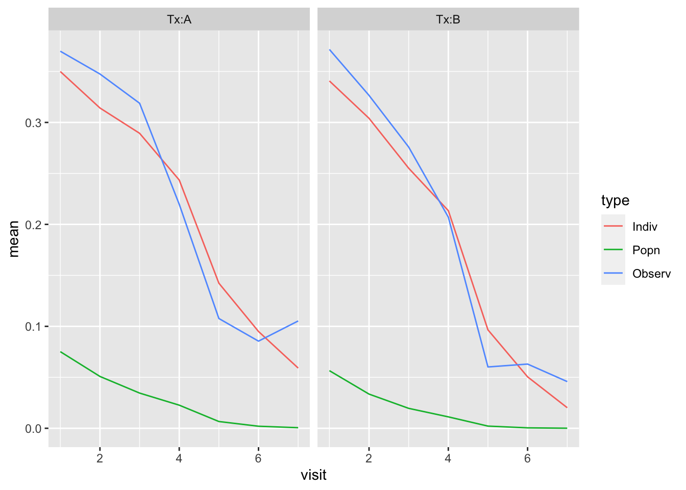
- You can see how fixed effects predictions are biased downward.
- Bringing the random effect back into the picture corrects the bias.
- NOTE: If we want to predict the probabilities of infection for a new individual, then the best prediction for \(\alpha\) is 0, yielding the fixed effect prediction (Why are we limited to this value for \(\alpha\)?)
5.2.9 The surprising results of fixed vs random effect based predicted probabilities
How do we understand the difference between averaged individual overall average effects? One way is to see that: \[ \mbox{expit}(E(Y|X))\neq E(\mbox{expit}(Y|X)) \] unless \(Y|X\) is symmetric about zero.
A simulation in which \(X=Y|X\) and \(X\sim N(1,1)\) will make the point:
Code
set.seed(2044)
X <- rnorm(10000, mean = 1, sd = 1)
Y <- locfit::expit(X)
expitMeanX <- locfit::expit(mean(X))
meanY <- mean(Y)
plot(density(Y), main = "expit(Y|X)")
abline(v = meanY, col = 8, lwd = 2)
abline(v = expitMeanX, col = 2, lwd = 2)
text(expitMeanX + 0.01, 0.5, "expit(E(Y|X))", adj = 0, col = 2)
text(meanY - 0.01, 0.5, "E(expit(Y|X))", adj = 1, col = 8)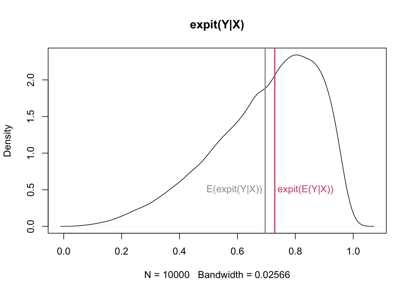
5.2.10 Estimation
- Maximum Likelihood Estimation
- The integral for the marginal likelihood requires a numerical approximation method.
- Gauss Hermite Quadrature is often used. You may be asked to specify the number of integration points. More is better, but slower.
- Generalized Estimating Equations
- A method that is often used to account for the dependence in the data by specifying a “working correlation matrix” as a surrogate for the true Cov(Y).
- Need some assumptions about the structure of the covariance matrix, such as exchangeability.
- If the working correlation close to the correct form, then it can be a useful approach.
- However assumptions about covariance are hard to verify and unfortunately the GEE results tend to be very sensitive to the structure of the working correlation (and missing data patterns).
- Bayesian Estimation: The posterior of \(\beta\) and \(\alpha\) can be computed easily as the likelihood function is given in terms of prior distributions of \(\beta\) and \(\alpha\), which form a natural hierarchical model.
- To make inference about \(\beta\) and \(\alpha\), we need to find a way to sample from the posterior distribution.
- If were are in what is known as a conjugate prior situation (such as Beta prior on a Binomial outcome), the posterior is a known distribution, so we can directly sample from it.
- If the posterior is not a closed form distribution, Bayesian computation methods such as MCMC and Gibbs sampler can be used to obtain random draws from the posterior distribution.
- Once you get the posterior draws of \(\beta\) and \(\alpha\), you can simply report the mean and standard deviation of the former, and the variance (for variance component) of the latter.
5.4 Coding
tapply()lmer()VarCorr()ranefglmer()
tapply()function is a part of apply family functions; it computes a function for each factor in a vector. It has arguments as follows:X: an object(vector)
INDEX: a list containing factor
FUN: a function applied to each element of X
Code
# compute mean of the mpg column grouped by cylinders
tapply(mtcars$mpg, mtcars$cyl, mean)
## 4 6 8
## 26.66364 19.74286 15.10000lmer()function is to fit a linear mixed-effects model to data fromlme4library. It has arguments as follows:formula: A 2-sided linear formula object; Random-effects terms are distinguished by vertical bars (|) separating expressions for design matrices from grouping factors. Two vertical bars (||) can be used to specify multiple uncorrelated random effects for the same grouping variable.
data: a dataframe containing the variables in the formula
REML: logical scalar
Detail information can be found with a link: https://www.rdocumentation.org/packages/lme4/versions/1.1-29/topics/lmer
Code
# load iris data
data(iris)
# fit the data with lmer function
fit <- lmerTest::lmer(sepal.len ~ sepal.wid + (1 | species), data = iris)
summary(fit)
## Linear mixed model fit by REML. t-tests use Satterthwaite's method ['lmerModLmerTest']
## Formula: sepal.len ~ sepal.wid + (1 | species)
## Data: iris
##
## REML criterion at convergence: 155.7
##
## Scaled residuals:
## Min 1Q Median 3Q Max
## -2.4618 -0.6130 -0.1451 0.6846 2.8646
##
## Random effects:
## Groups Name Variance Std.Dev.
## species (Intercept) 0.1055 0.3249
## Residual 0.2590 0.5089
## Number of obs: 100, groups: species, 2
##
## Fixed effects:
## Estimate Std. Error df t value Pr(>|t|)
## (Intercept) 3.6913 0.5192 19.7519 7.109 7.38e-07 ***
## sepal.wid 0.8951 0.1612 97.7284 5.554 2.41e-07 ***
## ---
## Signif. codes: 0 '***' 0.001 '**' 0.01 '*' 0.05 '.' 0.1 ' ' 1
##
## Correlation of Fixed Effects:
## (Intr)
## sepal.wid -0.891VarCorr()function calculates the estimated variance, standard deviation and correlation between the random-effects terms in a mixed-effects model, of class fromlme4library. It has arguments as follows:x: a fitted model object
sigma: a value used as a multiplier for the standard deviations
Detail information can be found with a link: https://www.rdocumentation.org/packages/lme4/versions/1.1-29/topics/VarCorr
Code
# compute the standard deviation between the random-effects term
lme4::VarCorr(fit)
## Groups Name Std.Dev.
## species (Intercept) 0.32485
## Residual 0.50887ranef()is a function to extract the random effects from a fitted model, also from thelme4library. It has arguments as follows:- object: an object of fitted models with random effects
Code
# extract the random effects
lme4::ranef(fit)
## $species
## (Intercept)
## versicolor -0.2237212
## virginica 0.2237212
##
## with conditional variances for "species"glmer()is a function to fit a generalized linear mixed-effects model from thelme4library. It has arguments as follows:formula: A 2-sided linear formula object; Random-effects terms are distinguished by vertical bars (
|) separating expressions for design matrices from grouping factors.family: a GLM family
Code
# fit a generalized linear mixed-effects model
fit.glmer <- lme4::glmer(outcome ~ time + treatment + (1 | patientID), family = binomial, data = toenail)
summary(fit.glmer)
## Generalized linear mixed model fit by maximum likelihood (Laplace Approximation) ['glmerMod']
## Family: binomial ( logit )
## Formula: outcome ~ time + treatment + (1 | patientID)
## Data: toenail
##
## AIC BIC logLik deviance df.resid
## 1267.6 1289.9 -629.8 1259.6 1904
##
## Scaled residuals:
## Min 1Q Median 3Q Max
## -3.7315 -0.1399 -0.0740 -0.0088 30.1542
##
## Random effects:
## Groups Name Variance Std.Dev.
## patientID (Intercept) 20.73 4.553
## Number of obs: 1908, groups: patientID, 294
##
## Fixed effects:
## Estimate Std. Error z value Pr(>|z|)
## (Intercept) -2.31940 0.74733 -3.104 0.00191 **
## time -0.46094 0.03963 -11.632 < 2e-16 ***
## treatmentterbinafine -0.68556 0.65901 -1.040 0.29821
## ---
## Signif. codes: 0 '***' 0.001 '**' 0.01 '*' 0.05 '.' 0.1 ' ' 1
##
## Correlation of Fixed Effects:
## (Intr) time
## time 0.280
## trtmnttrbnf -0.364 0.0815.5 Exercise & Quiz
5.5.1 Quiz: Exercise
- Use “Quiz-W5: Exercise” to submit your answers.
Describe a mechanism whereby students in the same classroom would have similar math test scores, e.g. Or pick another, non-repeated measures but nested design, and discuss how correlation is induced among observations in the same grouping unit.(link to exercise 1)
Describe some outcomes of interest that may be collected in a nested/longitudinal manner and why this design can be informative. Suggest possible \(X_{ij}\) and \(W_j\) and specify what \(i\) and \(j\) are.(link to exercise 2)
How might independence between students and among classrooms be violated in real data? Think about the many mechanisms for assigning children to schools/classrooms. What variables might be omitted in \(X\) and \(W\) perhaps because they are hard to measure? (link to exercise 3)
Discuss and explain: *why aren’t the lines exactly parallel? (link to exercise 4)
What does the plot tell us about individual differences? Why does it appear that only a few curves are drawn? (link to exercise 5)
What is wrong with taking the simple average of these points (by group) over time? HINT: is this a balanced, complete design? (link to exercise 6)
5.5.2 Quiz: R Shiny
Questions are from R shiny app “Lab 4: Longitudinal data”.
Use “Quiz-W5: R Shiny” to submit your answers.
Fit the model with
glmerfunction and find variables that are statistically significant (in fixed effects)Compute the mean of predictions using GLMMs
Compute the AIC value for three different fitted models
Compute the mean of two types of residuals (within and between) of
glm.glmmmodel.
5.5.3 Quiz: Chapter
Use “Quiz-W5: Chapter” to submit your answers.
Select a CORRECT sentence that describes the effect for the predictors (bill_length_mm)
First, fit the model with an interaction model (bill_length_mm*bill_depth_mm) and add parameter: maxit = 1000 when you run multinom. THEN Compute the confusion matrix for the model and report how many species do the models correctly predict overall (Please sum all correct cases).
Find a CORRECT Interpretation on the Infl coefficient as an odds ratio, being explicit about what is in the numerator and denominator of those odds. (You do not need to fit the model here)
Is there evidence of overdispersion (use deviance residuals and a chi-square test)
Interpret the bad health coefficient(“badh”) along with the proportion of non-user predicted by the model.
What is NOT a potential problem with clustered data?
What is NOT correct about the random effect?
Select the NOT correct interpretation about the summary of the linear mixed model.