Chapter 1 Chapter 1: Introduction to Generalized Linear Models (GLM)
Disclaimer: The causal aspect of statistical modeling is not the focus in this course.
Notation: we will use \(\log\) and \(\ln\) interchangeably (\(\log\) is understood as the natural logarithm).
1.1 Limited Dependent variables (LDVs)
When the outcome is limited in some way, such as always positive, discrete, ordinal, etc., we are in the realm of LDVs. Most methods you have used for modeling outcomes of interest were likely derived for normally distributed outcomes. Recall the linear regression assumption that errors are normal, e.g. Using the “wrong” model can yield a variety of problems, including:
- Biased coefficient estimates (compared to proper models)
- Predictions outside the range of the outcome
- Incorrect inference
1.1.1 Example: determinants of birth weights
Low birth weight, defined as birth weight less than 2500 grams (5.5 lb), is an outcome that has been of concern to physicians for years. This is due to the fact that infant mortality rates and birth defect rates are very high for low birth weight babies.
Behavior during pregnancy (including diet, smoking habits, and receiving prenatal care) can greatly alter the chances of carrying the baby to term and, consequently, of delivering a baby of normal birth weight.
We have a dataset that can help us understand the (correlational) relationship between certain mother characteristics and baby’s birthweight.
DSN: birthwt.dta (STATA13 format)

ID:         Mother's identification number
MOTH_AGE:   Mother's age (years)
MOTH_WT:    Mother's weight (pounds)
RACE:       Mother's race (1=White, 2=Black, 3=Other)
SMOKE:      Mother's smoking status (1=Yes, 0=No)
PREM:       History of premature labor (number of times)
HYPE:       History of hypertension (1=Yes, 0=No)
URIN_IRR:   History of urinary irritation (1=Yes, 0=No)
PHYS_VIS:   Number of physician visits
BIRTH_WT:   Birth weight of new born (grams)
In this case, we know the actual birthweight, but our interest is in the low birthweight status, which is a 0/1 (binary) outcome.
Let’s focus on available and constructed outcomes of interest and one risk factor:
- BIRTH_WT: Birth weight of new born (grams)
- LBW (constructed): Is the new born low birth weight (under 2500 grams).
- MOTH_AGE: Mother’s age (years)
What kind of statistical models we should use to “explore” the effects of risk factors on these outcomes? Next, we plot the relationship of each outcome to age, but in order to visualize the binary outcome, we have to make an interesting choice.
We begin with the continuous outcome, BIRTH_WT, and note that the linear relationship appears to be positive, by adding a default regression line.
Code
bwData <- readstata13::read.dta13("./Data/birthwt.dta", nonint.factors = TRUE)
bwData$LBW <- ifelse(bwData$BIRTH_WT < 2500, 1, 0)
ggplot(data = bwData, aes(y = BIRTH_WT, x = MOTH_AGE)) + geom_point(size = 0.6) + geom_smooth(method = "lm", formula = y ~
    x)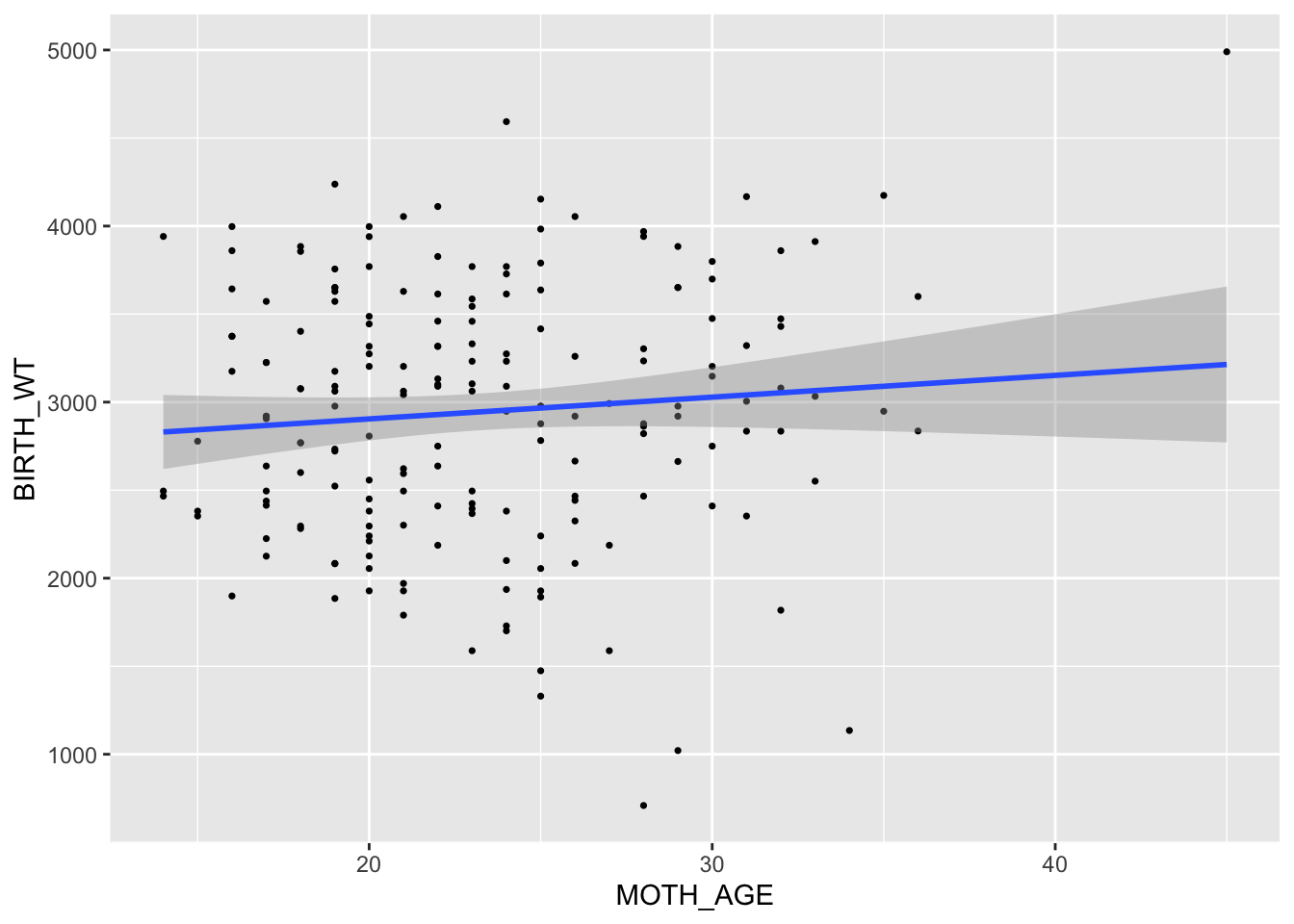
To visualize the binary (0/1) outcome, we choose to ‘jitter’ the values just a little bit on both the x and y axis. This should reveal the density, or frequency of points at each location. If we did not do this, all we will see is a single dot (here displayed as red circles) at each distinct (MOTH_AGE,LBW) pair.
Code
ggplot(data = bwData, aes(y = LBW, x = MOTH_AGE)) + geom_jitter(width = 0.2, height = 0.01, size = 0.6) + geom_point(shape = 16,
    size = 3, col = "red", alpha = 0.1, stroke = 0.1) + geom_smooth(method = "lm", formula = y ~ x)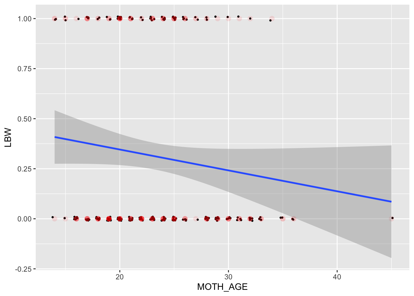
Code
# loess smooth would tell a whole other storyUnexpectedly, the apparent relationship is negative for LBW, while it is positive in the original scale (BIRTH_WT). One could say that this loss of information when we go from continuous to limited dependent is the root cause, but that ignores: clinical significance of low birth weight as an outcome; assumptions about the functional form (linear relationships with normally distributed errors).
In a linear model we expect the dependent variable \(Y\) and a predictor \(X\) to have a linear relationship, with normal errors: \[ Y_i = b_0 + b_1X_i + \varepsilon_i, \ \ \ \mbox{with }\varepsilon_i\sim N(0,\sigma^2) \]
Is this assumption reasonable when the outcomes are either 0 or 1? Clearly we have some challenges:
- How do we predict 0 or 1 when it appears that we predict on a continuous scale (thresholding at 0.50?)?
- Could we ever predict a negative value (answer: yes, but that’s bad)
- Assuming we predict only 0 or 1, then errors are either 0 or 1, but that’s not built into this framework at all.
Let’s examine the predictions made by these two linear models for a 20 year old mother:
Code
fit1 <- lm(data = bwData, BIRTH_WT ~ MOTH_AGE)
summary(fit1)
##
## Call:
## lm(formula = BIRTH_WT ~ MOTH_AGE, data = bwData)
##
## Residuals:
## Min 1Q Median 3Q Max
## -2294.53 -517.71 10.56 530.65 1776.27
##
## Coefficients:
## Estimate Std. Error t value Pr(>|t|)
## (Intercept) 2657.33 238.80 11.128 <2e-16 ***
## MOTH_AGE 12.36 10.02 1.234 0.219
## ---
## Signif. codes: 0 '***' 0.001 '**' 0.01 '*' 0.05 '.' 0.1 ' ' 1
##
## Residual standard error: 728 on 187 degrees of freedom
## Multiple R-squared: 0.008076, Adjusted R-squared: 0.002772
## F-statistic: 1.523 on 1 and 187 DF, p-value: 0.2188Code
pred1 <- predict(fit1, newdata = data.frame(MOTH_AGE = 20))
fit2 <- lm(data = bwData, LBW ~ MOTH_AGE)
summary(fit2)
##
## Call:
## lm(formula = LBW ~ MOTH_AGE, data = bwData)
##
## Residuals:
## Min 1Q Median 3Q Max
## -0.4085 -0.3355 -0.2625 0.6332 0.8001
##
## Coefficients:
## Estimate Std. Error t value Pr(>|t|)
## (Intercept) 0.554521 0.151724 3.655 0.000334 ***
## MOTH_AGE -0.010429 0.006367 -1.638 0.103083
## ---
## Signif. codes: 0 '***' 0.001 '**' 0.01 '*' 0.05 '.' 0.1 ' ' 1
##
## Residual standard error: 0.4625 on 187 degrees of freedom
## Multiple R-squared: 0.01415, Adjusted R-squared: 0.008875
## F-statistic: 2.683 on 1 and 187 DF, p-value: 0.1031Code
pred2 <- predict(fit2, newdata = data.frame(MOTH_AGE = 20))To be clear, we obtain predictions using the estimated coefficients from the regression models, \(\hat{b}_0\) and \(\hat{b}_1\). Given by this code:
Code
fit1$coefficients## (Intercept) MOTH_AGE
## 2657.33256 12.36433Code
fit2$coefficients## (Intercept) MOTH_AGE
## 0.55452107 -0.01042907These yield:
\(\widehat{BIRTH\_WT}\) = 2657.33 + 12.36(20) = 2904.62
and \(\widehat{LBW}\) = 0.55 + -0.01(20) = 0.35.
What are we to infer from these predictions? The latter is similar to a probability, although it is not constrained to be between 0 and 1.
1.1.1.1 Exercise 1
We need a more general modeling framework that can handle:
- Limited dependent variables (LDVs)
- Prediction within the range of the outcome
- Error structure that reflects the way in which data are generated (DGP=data generating process)
Examples of limited dependent variables:
- Binary(dichotomized) variable: smokers or not, often coded 0/1
- Ordinal and nominal variable: self-rated health, often coded 1/2/3/4, etc.
- Count variable: children ever born, takes only integer values 0,1,2,3,4,…
- Time to event variable: survival time >0
Generalized Linear Models (GLMs) provide a larger set of DGPs to handle the LDVs, such as those above.
Other limited dependent variables are censored and truncated variables:
- Truncation: very big or very small sample values are excluded from the sample.
- Censoring: very big or very small are compressed. E.g. one’s income is above $100,000, it is recoded as 100,000. Note: there are other meanings to the term censored.
There are different models that deal with these types of limited dependent outcomes; they are outside the generalized linear model framework.
1.2 Linear Models
Linear models have several appealing properties:
- Highly interpretable: coefficients (or slopes) may be called predictor effects; in the linear regression model, these represent the expected difference in outcomes between groups of individuals who differ by one unit on a single variable/predictor, and are otherwise identical.
- Inclusion of variables as controls for confounding is important scientifically.
- Interactions may be included easily in this framework.
- Non-linear relationships may be implemented through inclusion of polynomial terms, still maintaining the linear model framework (it is linear in the included variables, which may themselves be squared and higher order terms).
1.2.0.1 Exercise 2
To model limited dependent variables such as categorical and discrete variables, we will describe an extension of the linear model: \(Y=b_0 +b_1X_1+b_2X_2+\cdots+\varepsilon\) that allows us to use the same core linear form \(b_0 +b_1X_1+b_2X_2+\cdots+\) but adjusts the error structure and relationship to the outcome to handle the more general case.
In the rest of the semester, to keep the notation simple, we will sometimes exchange \(X\beta\) (the matrix form) for the linear sum, above. Note that in the matrix form, the first column of \(X\) is usually a vector of 1s to refect the constant in the model. Thus, \(X=(\mathbf{1},X_1,X_2,\cdots)\) and \(\beta=(b_0,b_1,b_2,\cdots)'\), then \(X\beta=1b_0 +b_1X_1+b_2X_2+\cdots\). It is important to note that \(X_1,X_2,\cdots\) are each column vectors, forming the matrix \(X\) and \(\beta\) is a column vector in this framework.
1.2.1 Linear regression under normal distribution assumption
In the linear model \(Y_i=X_i\beta +\varepsilon_i\), we don’t need to assume the distribution of the error term \(\varepsilon\). The least squares technique allows us to unbiasedly estimate \(\beta\). As long as \(\varepsilon\) is on average 0 (zero mean) and is independent from \(X\), when sample size is sufficiently large, the behavior of these estimators is well understood.
However, if we further assume \(\varepsilon\) is normally distributed with mean 0 and variance \(\sigma^2\), things can become a little bit more interesting:
\(Y_i=X_i\beta +\varepsilon_i\) and \(\varepsilon\sim N(0,\sigma^2)\) implies that given \(X\), \(Y\) is normally distributed with mean \(\mu_i\) and variance \(\sigma^2\), where \(\mu_i = X_i\beta\) is the conditional mean, given \(X\). Notationally, \(Y_i | X_i,\sigma^2 \sim N(\mu_i,\sigma^2)\).
The distributional assumption allows us to make further inference about the regression parameters (slopes) as well.
Example: Using the simple linear regression model of birth weight on mother’s age, the birth weights of babies born to 20-year old mothers have a normal distribution with mean 2904.62 grams. In this case, \(\mu_i\)=2904.62 for \(X_i\)=20 (\(X\) is mother’s age).
We now generalize linear regression by looking at all of the components of the model and how they relate to each other. This will allow us to generalize to limited dependent variables.
1.3 Generalizing linear regression to GLM
In a generalized linear modeling (GLM) setting, we need to specify:
- How data are generated; the family of distributions from which observations are drawn, and the parameters governing that distribution.
- How a general set of parameters are related to variables/predictors through a linear model.
- How the parameters governing the distribution are related to the DGP.
For linear regression, we have \(\mu_i=X\beta\), \(\sigma^2\) is a constant (does not depend on \(\mu_i\) or \(X\)) and \(Y_i|X_i,\sigma^2 \sim N(\mu_i,\sigma^2)\)
In terms of the GLM components:
- \(Y_i|\mu_i,\sigma^2 \sim N(\mu_i,\sigma^2)\)
- \(\eta_i=X_i\beta\) (using notation \(\eta\) allows it to be more general).
- \(E(Y_i|X_i)=\mu_i=g^{-1}(\eta_i)=\eta_i\) (g is called an identity link - nothing changes). \(\sigma^2\) does not vary.
The key aspect of this framework is that the linear model only sets a parameter \(\eta\), which then must be related to the conditional mean of the DGP. The link function (\(g^{-1}(\cdot)\)) relates \(\eta\) to the central parameter of the DGP, which is usually a mean or rate. The definition in terms of the inverse will be important subsequently.
1.4 The Data Generating Process (DGP)
A DGP is a model and a procedure for generating data. It can be thought of as an approximation to whatever social or physical process gives rise to observed data. It contains an error term of some type, either representing variability due to imprecise measurement, our inability to measure all of the important factors generating the observation, or simply natural variation in the population.
Example: Suppose we intend to measure mother’s age in years (\(X_i\)) and baby’s birthweight in grams (\(Y_i\)) and relate them in a linear manner. We might posit the following relationship:
\[ Y_i=2500 + 15 X_i +\varepsilon_i \] with \(\varepsilon_i\sim N(0,700^2)\). We can look at what this model implies for the type of data expected by generating a few observations:
Code
set.seed(2044001)
N <- 20
X <- seq(20, 40, length = N)
eps <- rnorm(N, sd = 700)
Y <- 2500 + 15 * X + eps
dta <- tibble::tibble(X = X, Y = Y)
dta
ggplot(dta, aes(x = X, y = Y)) + geom_point()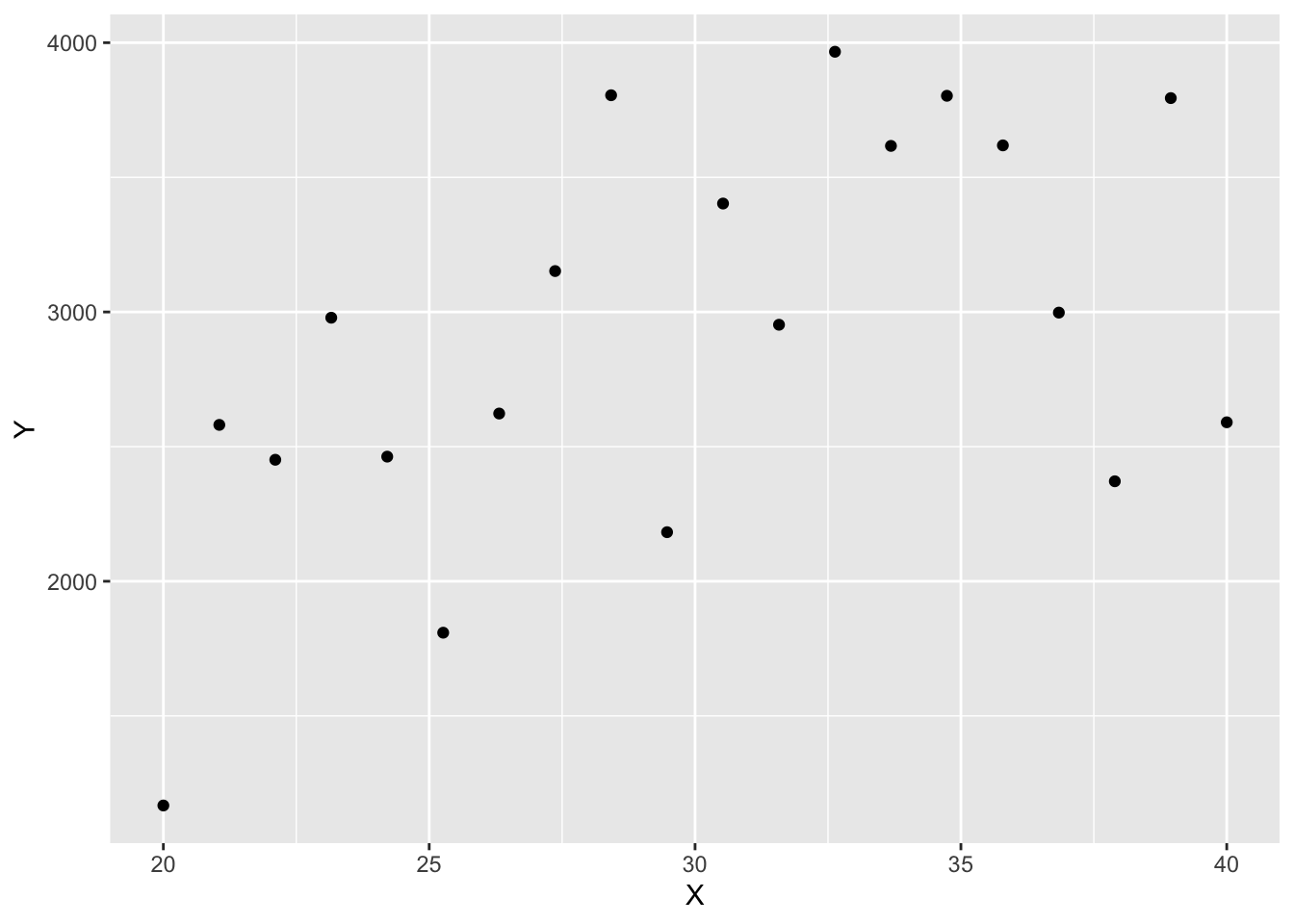
Extension: We can extend the prior DGP, generating a different outcome – whether a baby is low birthweight (<2500 grams; as \(Z_i\)) by thresholding the observation. In other words, we set
\[ Z_i= \left\{ \begin{array}{ c l } 0 & \quad \textrm{if } Y_i > 2500 \\ 1 & \quad \textrm{otherwise} \end{array} \right. \] This DGP generates binary outcomes by thresholding a birthweight from the prior DGP. We can eliminate this intermediate step using a clever transform. Use of transforms are central to GLMs.
We can convert a probability \(p_i\in (0,1)\) to a real number in \(Y_i\in (-\infty, +\infty)\) using the logit transform: \(Y_i=\log(p_i/(1-p_i))\). When \(p_i<0.5\), \(Y_i<0\) and when \(p_i>0.5\), \(Y_i\ge 0\). The inverse of the logit transform is called expit and may be written: \[ \textrm{expit}(z) = \frac{e^{z}}{1+e^{z}} \] You can confirm that \(\textrm{expit}(\textrm{logit}(p))=p\)
Example: We measure mother’s age in years (\(X_i\)) and whether the baby is low birthweight (\(Z_i\)) and relate \(X_i\) to \(Z_i\) in a nonlinear manner, through a logit transform and a different random process.
\[ logit(p_i)=0.40 -0.05 X_i \] \[ Z_i \sim \textrm{binomial}(p_i) \] We can look at what this model implies by generating a few observations:
Code
set.seed(2044001)
expit <- function(z) {
    exp(z)/(1 + exp(z))
}
N <- 20
X <- seq(20, 40, length = N)
p <- expit(0.4 - 0.05 * X)
Z <- rbinom(N, 1, prob = p)
dta <- tibble::tibble(X = X, Z = Z)
dta
1.4.1 GLM Examples, with their components:
Logistic regression:
- \(Y_i \sim \mbox{binom}(p_i)\) (Note: without loss of generality, we refer to a binomial, but in most instances it is a single draw and is thus a Bernoulli on the outcome space 0/1). \(p_i=E(Y_i|X_i)\)
- \(\eta_i = X_i\beta\) (linear component)
- \(g(p_i) = log\left(\frac{p_i}{1-p_i}\right)=\eta_i\), thus \(g^{-1}(\eta_i)=\left(\frac{\exp(\eta_i)}{1+\exp(\eta_i)}\right)\), the so-called logit and expit functions, respectively.
Note: the logit link transforms a probability to the full space \(\Re\), allowing the linear model portion to range from \(-\infty\) to \(+\infty\). Or conversely, the inverse, or expit function transforms \(\Re\) to \((0,1)\). From either perspective it allows us to impose a linear model when the outcome is 0/1. This is very elegant!
In fact, it is acceptible to write a logistic model as follows, using the \(g^{-1}\) function in a reasonable way:
\[
Y_i \sim \mbox{binom}\left(\frac{e^{X_i\beta}}{1+e^{X_i\beta}}\right)
\]
Note: the binom distribution here is understood as Bernoulli for a single observation.
If you need to brush up your understanding about probability distributions such as binomial distribution and Poisson distribution, you can take a look at –>
1.5 Exponential Family of Distributions
The Generalized Linear Models were formally developed by McCullagh and Nelder (1989). They specifically refer to dependent variables that follow a family of distributions called the Exponential family distribution. The basic form of the natural exponential family (single parameter in canonical form; a subset) has the following p.d.f.:
\[ f_Y(y|\theta) = h(y)\exp(\theta y -A(\theta)) \] where \(h(y)\) and \(A(\theta)\) are known functions, \(\theta\) is a scalar here, but may be a vector in more general forms.
1.5.1 Why exponential family?
For this class of models, the maximum likelihood estimates (MLEs) can all be obtained using the same iterative algorithm. Also, it may seem surprising at first, but normal (Gaussian), Bernoulli and binomial, Poisson, and many other distributions can be written in this manner or its minor extensions, through some algebraic manipulation.
For the Bernoulli/binomial, \(f_Y(y|p)=p^y(1-p)^{1-y}\). We show that with the following set of definitions, this is in the exponential family. Let \(\theta=\log\frac{p}{1-p}\), \(h(y)=1\), and \(A(\theta)=\log(1+e^\theta)\), then: \[\begin{eqnarray*} f_Y(y|p) & = & \exp(y\theta - \log(1+e^\theta)) \\ & = & \frac{(\exp{\theta})^y}{1+\exp\theta} \\ & = & \frac{(\frac{p}{1-p})^y}{1+\frac{p}{1-p}} \\ & = & \frac{p^y(1-p)^{-y}(1-p)^1}{(1-p)+(p)} \\ & = & p^y(1-p)^{1-y} \end{eqnarray*}\]
In the table below, we list the members of the exponential family distributions that we consider in this course, and related link functions.
It is important to understand that the link functions are applied to parameters of the model, not to the outcomes directly.
- With logit models, e.g., we are not modeling the logit of the outcome, but rather the logit of the probability of the outcome.
- With Poisson regression, we are not modeling the log of the count, but rather the log of the underlying rate of activity that leads to a count.
1.6 Quick look at GLM in R
The R function glm can be thought of as an extension of lm and allows the user to specify the family and link in the family parameter. We explore the relationship between child being born low birthweight (in one instance, just birthweight) with mother’s age in three different GLMs, below:
Code
fit.bw.norm <- glm(BIRTH_WT ~ MOTH_AGE, data = bwData, family = gaussian(link = "identity"))
fit.lbw.norm <- glm(LBW ~ MOTH_AGE, data = bwData, family = gaussian(link = "identity"))
fit.lbw.logit <- glm(LBW ~ MOTH_AGE, data = bwData, family = binomial(link = "logit"))
fit.lbw.probit <- glm(LBW ~ MOTH_AGE, data = bwData, family = binomial(link = "probit"))
fit.lbw.pois <- glm(LBW ~ MOTH_AGE, data = bwData, family = poisson(link = "log"))  #very odd choice

summary(fit.bw.norm)
##
## Call:
## glm(formula = BIRTH_WT ~ MOTH_AGE, family = gaussian(link = "identity"),
## data = bwData)
##
## Deviance Residuals:
## Min 1Q Median 3Q Max
## -2294.53 -517.71 10.56 530.65 1776.27
##
## Coefficients:
## Estimate Std. Error t value Pr(>|t|)
## (Intercept) 2657.33 238.80 11.128 <2e-16 ***
## MOTH_AGE 12.36 10.02 1.234 0.219
## ---
## Signif. codes: 0 '***' 0.001 '**' 0.01 '*' 0.05 '.' 0.1 ' ' 1
##
## (Dispersion parameter for gaussian family taken to be 530000.7)
##
## Null deviance: 99917053 on 188 degrees of freedom
## Residual deviance: 99110126 on 187 degrees of freedom
## AIC: 3031.5
##
## Number of Fisher Scoring iterations: 2Code
summary(fit.lbw.norm)##
## Call:
## glm(formula = LBW ~ MOTH_AGE, family = gaussian(link = "identity"),
## data = bwData)
##
## Deviance Residuals:
## Min 1Q Median 3Q Max
## -0.4085 -0.3355 -0.2625 0.6332 0.8001
##
## Coefficients:
## Estimate Std. Error t value Pr(>|t|)
## (Intercept) 0.554521 0.151724 3.655 0.000334 ***
## MOTH_AGE -0.010429 0.006367 -1.638 0.103083
## ---
## Signif. codes: 0 '***' 0.001 '**' 0.01 '*' 0.05 '.' 0.1 ' ' 1
##
## (Dispersion parameter for gaussian family taken to be 0.2139461)
##
## Null deviance: 40.582 on 188 degrees of freedom
## Residual deviance: 40.008 on 187 degrees of freedom
## AIC: 248.9
##
## Number of Fisher Scoring iterations: 2Code
summary(fit.lbw.logit)##
## Call:
## glm(formula = LBW ~ MOTH_AGE, family = binomial(link = "logit"),
## data = bwData)
##
## Deviance Residuals:
## Min 1Q Median 3Q Max
## -1.0402 -0.9018 -0.7754 1.4119 1.7800
##
## Coefficients:
## Estimate Std. Error z value Pr(>|z|)
## (Intercept) 0.38458 0.73212 0.525 0.599
## MOTH_AGE -0.05115 0.03151 -1.623 0.105
##
## (Dispersion parameter for binomial family taken to be 1)
##
## Null deviance: 234.67 on 188 degrees of freedom
## Residual deviance: 231.91 on 187 degrees of freedom
## AIC: 235.91
##
## Number of Fisher Scoring iterations: 4Code
summary(fit.lbw.probit)##
## Call:
## glm(formula = LBW ~ MOTH_AGE, family = binomial(link = "probit"),
## data = bwData)
##
## Deviance Residuals:
## Min 1Q Median 3Q Max
## -1.0413 -0.9030 -0.7737 1.4102 1.7903
##
## Coefficients:
## Estimate Std. Error z value Pr(>|z|)
## (Intercept) 0.23590 0.43981 0.536 0.5917
## MOTH_AGE -0.03155 0.01875 -1.682 0.0925 .
## ---
## Signif. codes: 0 '***' 0.001 '**' 0.01 '*' 0.05 '.' 0.1 ' ' 1
##
## (Dispersion parameter for binomial family taken to be 1)
##
## Null deviance: 234.67 on 188 degrees of freedom
## Residual deviance: 231.85 on 187 degrees of freedom
## AIC: 235.85
##
## Number of Fisher Scoring iterations: 4Code
summary(fit.lbw.pois)##
## Call:
## glm(formula = LBW ~ MOTH_AGE, family = poisson(link = "log"),
## data = bwData)
##
## Deviance Residuals:
## Min 1Q Median 3Q Max
## -0.9240 -0.8154 -0.7196 0.8535 1.2446
##
## Coefficients:
## Estimate Std. Error z value Pr(>|z|)
## (Intercept) -0.35138 0.60202 -0.584 0.559
## MOTH_AGE -0.03571 0.02635 -1.355 0.175
##
## (Dispersion parameter for poisson family taken to be 1)
##
## Null deviance: 137.38 on 188 degrees of freedom
## Residual deviance: 135.46 on 187 degrees of freedom
## AIC: 257.46
##
## Number of Fisher Scoring iterations: 51.6.0.1 Exercise 3
In GLM, the mean of the outcome variable \(Y\) is specified as a function of \(X\beta\), so we can still interpret the effect of \(X\) on \(Y\) in terms of the components of \(\beta=(b_0,b_1,\ldots,b_k)\) for a model with \(k\) predictors. Let us focus on the effect of \(X_1\), say \(b_1\), that we estimate.
In linear regression, we say that \(b_1\) is the difference in expected outcomes for values of \(X_1\) that differ by one unit. \(E(Y|X_1=x+1,X_2,\ldots,X_k)-E(Y|X_1=x,X_2,\ldots,X_k)\) holding \(X_2,\ldots,X_k\) constant in this case.
In logistic regression, we have to interpret a bit differently. Either \(b_1\) is the difference in expected log-odds for the probability of outcome 1, or \(e^{b_1}\) is the multiplicative factor for the expected odds for the outcome 1, again holding all other included variables constant. We provide a few details here:
- Let \(E(\log[\frac{p}{1-p}]|X_1=x+1,X_2,\ldots,X_k)\) be given by \(\log[\frac{p_1}{1-p_1}]\) and similarly by \(\log[\frac{p_0}{1-p_0}]\) for \(X_1=x\).
- The difference in expectations, exponentiated, is: \[ \begin{aligned} e^{\log[\frac{p_1}{1-p_1}]}-e^{\log[\frac{p_0}{1-p_0}]} = \frac{e^{\log[\frac{p_1}{1-p_1}]}}{e^{\log[\frac{p_0}{1-p_0}]}} = e^{b_1} \end{aligned} \]
- This reduces to: \[ e^{b_1}=\frac{\frac{p_1}{1-p_1}}{\frac{p_0}{1-p_0}} \] which is called the odds-ratio.
- The multiplicative interpretation is derived from the fact that if the original odds of a 1 outcome were \(\frac{p_0}{1-p_0}\), then the new expected odds, when \(X_1\) changes by one unit, holding all else constant, are: \[ e^{b_1}\frac{p_0}{1-p_0}=\frac{\frac{p_1}{1-p_1}}{\frac{p_0}{1-p_0}}\cdot\frac{p_0}{1-p_0} = \frac{p_1}{1-p_1} \] We will give examples of this interpretation in subsequent handouts.
1.7 Likelihood and Maximum Likelihood Estimation
We can estimate the parameters in our model, typically the \(\beta\) vector, using Maximum Likelihood estimation procedures.
1.7.1 What is Likelihood?
If we assume that the outcomes are generated from a certain probability distribution \(f_Y(\cdot\vert\theta)\), such as normal or binomial, we can evaluate the density (or loosely spoken, “probability”, or likelihood) of observing the \(Y\) under different values of \(\theta\), which would be \(f_Y(Y\vert\theta)\).
The likelihood is a “reverse-perspective” version of the p.d.f. It takes the data to be given and evaluates different values of \(\theta\). Thus it is viewed as a function of \(\theta\) given data \(Y\), and we write it \(L(\theta\vert Y,\ldots)\). The \(\ldots\) could be other data values that are also conditioned upon, such as \(X\).
1.7.2 Normal example:
\[ f(Y|\mu ,\sigma )=\frac{1}{\sqrt{2\pi {{\sigma }^{2}}}}{{e}^{-\frac{{{(Y-\mu )}^{2}}}{2{{\sigma }^{2}}}}} \] This is the density function of a (univariate) normal distribution with mean \(\mu\) and variance \(\sigma^2\).
The density evaluated at \(Y=1\) for an \(N(\mu=0,\sigma^2=1)\) distribution is
\[
\frac{1}{\sqrt{2\pi }}{{e}^{-\frac{1}{2}}}=0.242
\]
Thus, we can say that the likelihood, \(L(\mu=0,\sigma^2=1|Y=1)\) is \(0.242\).
The likelihood of \(\mu=1,\sigma^2=1\) given observation \(Y=1\) is \[ \frac{1}{\sqrt{2\pi }}{{e}^{0}}=0.399 \]
Thus we say that \(\mu=1\) is more likely than \(\mu=0\), given the data \(Y=1\). Of course, you can also say that it is more likely to observe the value 1 under normal distribution with mean 1 than the one with mean 0, but be careful, \(Y=1\) is held fixed, so the different mean parameters \(\mu\) are what is being compared as more or less likely (to have generated the given data).
1.7.2.1 Exercise 4
Note that in GLM, we have gone to great effort to relate the mean parameters to a set of predictors, \(X\), which are also data. Thus, in the linear regression case, with \(\mu=X\beta\), the parameters of interest will be (\(\beta\), \(\sigma^2\)), as these, along with the definition of \(\mu\) fully specify a normal likelihood.
1.7.3 Maximum Likelihood Estimation
Maximum Likelihood Estimation (MLE) is a procedure of finding the set of parameter values that are most consistent with the observed data, with the likelihood as the “judge” of consistency. We appeal to the likelihood to choose between alternative values of the parameters, and the MLE is the set of parameters that maximize it.
Quick example: return to the single observation \(Y=1\) from a normal distribution. The likelihood is:
\[ L(\mu|Y,\sigma)=f_Y(Y|\mu,\sigma)=\frac{1}{\sqrt{2\pi}\sigma}e^{-\frac{(Y-\mu )^{2}}{2\sigma^2}} \] Let us say that we know the variance \(\sigma^2=1\). Then this reduces to: \[ L(\mu|Y)=\frac{1}{\sqrt{2\pi}}e^{-\frac{1}{2}(Y-\mu)^2} \] It is often advantageous to take logs, and this does not change the maximization problem, because log is a monotonic transform (order preserving). We do this, to reveal the log-likelihood, often denoted with a lowercase script \(\ell\):
\[ \ell(\mu|Y)= - \frac{1}{2} \log(2\pi)-\frac{1}{2}(Y-\mu)^2 \] The MLE is the maximizer of \(\ell(\mu|Y)\); the first term in that expression clearly does not vary with \(\mu\), so the MLE is obtained as: \[ \min_\mu \frac{1}{2}(Y-\mu)^2 \] and recall that \(Y\) is given. From calculus, take the first derivative of this expression with respect to \(\mu\) and set it equal to zero: \(Y-\mu=0\), thus the MLE, denoted \(\hat\mu\) is given by \(Y\) in this instance. So the MLE for \(\mu\) given known variance 1 and observed value \(Y=1\), is \(\hat\mu=1\). This occurs because there is only one value. Were there multiple values, a bit more work would be required, but not much.
In practice, there are \(n\) sample data points, and we want to find the parameter values under which distribution we maximize the likelihood of jointly observing the data. If we assume the data points are all independent from each other, the joint likelihood is formed as the product, and the joint log-likelihood as the sum. The MLE estimator maximizes the joint likelihood:
\[ L(\theta |\vec{Y})=(Y_1,Y_2,\ldots,Y_n)')=\prod\limits_{i=1}^{n}{f_Y(Y_i|\theta)} \]
or the joint log-likelihood:
\[ \ell(\theta |\vec{Y})=\sum\limits_{i=1}^{n}{\log f_Y({{Y}_{i}}|\theta )} \]
As stated earlier, if a certain value of \(\theta\) maximizes \(L\), then it also maximizes \(\ell\), since the logarithm function is a monotonic transformation. Working with log-likelihood is better since we don’t have to deal with the products (both to avoid computational overflow and for mathematical elegance - e.g., when taking derivatives).
As alluded to in the quick example, mathematically, the MLE estimate of \(\theta\) may be found by taking first partial derivative of \(\ell\) with respect to (each element of ) \(\theta\) and solve equation(s) \(\frac{\partial l}{\partial \theta }=0\). Solving for \(\hat{\theta}\) is not always an easy task. It often requires iterative estimation procedure, such as Newton Raphson, Fisher Scoring and Iteratively reweighted least squares (IRLS). And as implied, \(\theta\) may be multidimensional, resulting in what are called the “score equations.”
1.7.4 Normal-linear regression example:
We denote the likelihood by \(L\) but note that it is a function of the data and parameters. The data are \(Y\) and \(X\), while the parameters are \(\sigma^2\) and either \(\mu\) or \(X\beta\), since we have a linear expression for \(\mu=X\beta\), the \(\mu\) parameter is replaced by \(X\beta\):
\[ \begin{aligned} L=\prod\limits_{i=1}^{n}{\frac{1}{\sqrt{2\pi\sigma^2}}{e^{-\frac{(Y_i-\mu )^2}{2\sigma ^2}}}}=(2\pi\sigma^2)^{-n/2}e^{-\frac{1}{2\sigma^2}\sum_{i=1}^{n}{(Y_i-\mu)^2}}=(2\pi\sigma^2)^{-n/2}e^{-\frac{1}{2\sigma^2}\sum_{i=1}^{n}{(Y_i-X_i\beta)^2}} \end{aligned} \]
and the log-likelihood is:
\[ \begin{aligned} \ell=-\frac{n}{2}\log 2\pi -\frac{n}{2}\log {{\sigma }^{2}}-\frac{1}{2\sigma ^2}\sum\limits_{i=1}^{n}{{{({{Y}_{i}}-{{X}_{i}}\beta )}^{2}}} \end{aligned} \]
Plugging in observed \(Y_i\) and \(X_i\) values, \(i=1,\ldots,n\), we look for values of \(\beta\) and \(\sigma\) that maximizes the log-likelihood \(\ell\) by solving:
\[ \frac{\partial \ell}{\partial \vec\beta }=\vec 0 \mbox{ and }\frac{\partial \ell}{\partial {{\sigma }^{2}}}=0 \] The notation \(\vec\beta\) reminds us that \(\beta\) is a vector, so the first equation represents a set of equations.
The solutions, denoted \(\vec{\hat{\beta}}\) and \({{\hat{\sigma}}^{2}}\)are the maximum likelihood estimator of \(\vec\beta\) and \(\sigma^2\).
As it turns out, in the normal-linear regression case, the MLE estimator of \(\beta\) is the same as least squares estimator, while the MLE estimator of \(\sigma^2\) is slightly biased (by a factor of \(n/(n-1)\)).
It is worth seeing how we can solve for the MLE in the case of simple linear regression, in which \(\beta=(b_0,b_1)\) and there is only one predictor \(X\).
1.7.5 Solve for \(\hat\sigma^2\)
\[ \frac{\partial \ell}{\partial\sigma^2}=-\frac{n}{2}\frac{1}{\sigma^2}+\frac{1}{2(\sigma ^2)^2}\sum\limits_{i=1}^{n}{{{({{Y}_{i}}-{{X}_{i}}\beta )}^{2}}}=0 \] \[ \implies \hat\sigma^2=\frac{1}{n}\sum\limits_{i=1}^{n}{(Y_i-X_i\beta)^2} \] We don’t know \(\beta\) yet, but once we have MLEs for it, we have an estimator for the MLE for \(\sigma^2\) with the above formula.
\[ \frac{\partial \ell}{\partial b_0}=\frac{1}{2\sigma^2}\sum\limits_{i=1}^{n}{2(Y_i-X_i\beta)^1}=0 \implies \sum\limits_{i=1}^{n}{[Y_i-(b_0+b_1X_i)]}=0 \] \[ \implies \sum\limits_{i=1}^{n}{Y_i}= nb_0+b_1\sum\limits_{i=1}^{n}{X_i}\implies \hat{b}_0 = \bar{Y}-\hat{b}_1\bar{X} \] Lastly,
\[ \begin{aligned} \frac{\partial \ell}{\partial b_1}=\frac{1}{2\sigma^2}\sum\limits_{i=1}^{n}{2(Y_i-X_i\beta)X_i}=0 \implies \sum\limits_{i=1}^{n}{[Y_iX_i-(b_0+b_1X_i)X_i]}=0 \end{aligned} \] While it is a bit more work to simplify this expression, we will show only one more step: \[ \begin{aligned} \implies \sum\limits_{i=1}^{n}{X_iY_i}=nb_0\bar{X}+b_1\sum\limits_{i=1}^{n}{X_i^2}\implies \hat{b}_1 = \left[\sum\limits_{i=1}^{n}{X_iY_i}-nb_0\bar{X}\right] \bigg/ \sum\limits_{i=1}^{n}{X_i^2} \end{aligned} \]
While this looks complicated, all of the terms may be directly calculated from \(X\) and \(Y\), and thus there are 3 equations and 3 unknowns. You will get a familiar expression, eventually.
1.8 Inferential tests and model evaluation for GLM
1.8.1 Hypothesis Testing
In many applications, interest centers on the regression parameters given by \(\beta\). Researchers wish to know whether predictors have effects beyond those expected by chance. This leads naturally, in a frequentist inferential framework, to hypothesis tests such as:
\(H_0\): \(b_1=0\) vs. \(H_a\): \(b_1\neq 0\)
In this one-dimensional case, we can use a z-test or t-test; we have the s.e. from asymptotic theory, as just described.
When interest lies in a larger predictor set, such as those generated by a set of indicator variables, we can form more complex hypotheses:
\(H_0\): \(\vec\beta=\vec 0\) vs. \(H_a\): \(\vec\beta\neq \vec 0\)
Here we use \(\vec\beta\) to refer to a set of regression coefficients to be tested. \(H_a\) is to be interpreted as “not all effects are statistically zero.”
The simplest version of the Wald test allows us to test this joint hypothesis:
\[ W=\hat\beta'\Sigma^{-1}\hat\beta \sim \chi^2_k \] is the Wald test statistic for the joint null, with \(\hat\beta\) a column vector (thus the prime symbol will make it a \(k\times 1\) row vector), and \(\hat\Sigma\) the asymptotic var-cov matrix of the parameter estimators. It has an asymptotic Chi-square distribution on \(k\) (the number of elements in \(\hat\beta\)) degrees of freedom.
More complex linear hypotheses, such as:
\(H_0\): \(L\vec\beta=\vec 0\) vs. \(H_a\): \(L\vec\beta\neq \vec 0\),
where \(L\) is a linear contrast, such as \(L=(1,0,-1)\), in which the first element of the vector is contrasted with the third, can also use a more complex form of the Wald test.
In one dimensional case (k=1), the Wald test statistic reduces to a z-test, as a chi-square distribution is a squared standard normal.
1.8.2 Likelihood Ratio Test (LRT)
Under the ML framework, sequential, nested models can be compared using likelihood ratio test statistics. Theory states that if two models, M0 and M1 are nested, meaning M1 contains all of the predictors in M0, then the differences in log-likelihoods,\(-2(\log L_1-\log L_0)\sim\chi^2_p\), where \(p\) is the number of unique predictors/parameters in model M1.
Another way to understand this test is that similar to \(R^2\) in linear regression, the likelihood increases as we include more predictors in the model. The LRT is to test whether the increment in likelihood due to the inclusion of new parameters is sufficiently large to reject the null that all of those additional parameters are zero.
1.8.3 Model Evaluation
How well does the model fit the data? In linear regression, \(R^2\) is one measure. It explains the percentage of the variability in \(Y\) being explained by \(X\) (the model). When the model fits the data perfectly, i.e. each Y value is perfectly predicted given the corresponding \(X\) value, \(R^2=1\).
The Deviance statistic is one such measure for Generalized Linear Models. If we use \(Y\) as predictor for the dependent variable (this may seem odd, but think of it instead as including indicators for each unique record), then the highest possible likelihood is obtained among all possible models, such value is called likelihood under the full or saturated model (\(L_s\)). The deviance statistic for a model (model A) with a set of predictors \(X\) is \(2(\log L_s - \log L_A)\), or an LRT for your model A vs. the saturated (best) model. How far are you from the best model, in other words?
The smaller the deviance statistic, the better the model fits the data. The Deviance statistic follows a Chi-square distribution with df=\(n-p\), with \(p\) as the number of parameter in model A. We can construct a deviance based goodness-of-fit test:
\(H_0\): Model A fits the data as well as the full model
\(H_a\): Model A does not fit the data as well as the full model.
and the LRT\(\sim\chi^2_{n-p}\) applies.
1.8.4 Residuals diagnosis
Let \(\hat\mu_i\) denote the prediction for the \(i^{th}\) case throughout this discussion.
Deviance residual (based on direct evaluation of the likelihood): \[ r_{Di} = 2[\log L(Y_i|\mbox{data})-\log L(\hat\mu_i|\mbox{data})] \]
Pearson’s residual (similar to standardized residual in linear regression), is useful when variance is a function of the mean, as it is in logistic and Poisson regression, among others. \[ r_{Pi}=\frac{y_i-\hat{\mu}_i}{\sqrt{V(\hat{\mu}_i)}} \]
Anscombe residual (they are more normally distributed residuals) \[ r_{Ai}=\frac{A(y_i)-A(\hat{\mu}_i)}{A'(\hat{\mu}_i)\sqrt{V(\hat{\mu}_i)}} \] where \(A(\mu)=\int_{-\infty}^\mu V^\frac{1}{3}(t)dt\), and \(A'\) is its derivative. The transform is non-trivial when variance is a function of level (non-normal outcomes).
1.8.5 Model Selection
To select between nested models, we can use LRT to test whether additional \(\beta\) parameters are statistically significantly different from 0.
When models are not nested, we can use likelihood based model selection criterion.
AIC = \(-2\log L+2p\)
BIC = \(-2\log L+ p\log(n)\)
where \(p\) is the number of predictors in the model.
When comparing two models, smaller AIC/BIC values are preferred. Both criteria are constructed as the negative log-likelihood plus a value that increases with model size (in order to penalize model size).
AIC and BIC do not always agree. BIC is the more conservative one (prefers the smaller model, fewer number of predictors), it puts a bigger penalty on model size because \(p\log(n)>2p\) when sample size \(n>8\).
1.9 Appendix
1.9.1 GLM Examples: Poisson regression
The count outcome variable \(Y_i\) follows a Poisson distribution with mean parameter \(\lambda_i\), conditioned on \(X_i\), but how do we relate these components? You might have seen Poisson regression written \(\log(E(Y|X))=X\beta\), reflecting that the mean of the Poisson process is modeled as a linear function of \(X\). It is important to note that we do not observe \(E(Y|X)\) but rather \(Y\), and thus we must find a way to connect all of the pieces correctly. This is why we have a link function.
- \(Y_i \sim \mbox{Pois}(\lambda_i)\), and note that for a Poisson process, \(Y\), \(E(Y)=V(Y)=\lambda\) (the mean and variance are the same – the value of the rate parameter).
- \(\eta_i = X_i\beta\) (linear component; should look very familiar by now)
- \(g(\lambda_i)=\log\lambda_i\), so \(g^{-1}(\eta_i)=\exp(\eta_i)\)
In fact, it is acceptible to write a Poisson model as follows, using the \(g^{-1}\) function in a reasonable way: \[ Y_i\sim \mbox{Pois}(e^{X_i\beta}) \] The inverse logarithm transforms the rate into the range \(\Re^+\), which is essential (there are no negative rates).
1.9.2 Standard error estimation
To estimate the standard error of MLE for the general parameter \(\hat{\theta}\), asymptotic (large sample) theory tells us that we can use the inverse of the Fisher Information. Fisher Information (\(I(\hat\theta)\)) is based on the second partial derivative(s) of the log-likelihood function (also called the Hessian, \(H\)). Note that in all but the simplest case, this is a matrix of partial derivatives. For example, for the simple linear regression model (\(Y_i=b_0+b_1+\varepsilon_i\), with \(\varepsilon_i\sim N(0,\sigma^2)\)), construct the Hessian:
\[ H= \begin{bmatrix} \frac{\partial \ell^2}{\partial b_0^2} & \frac{\partial \ell^2}{\partial b_0\partial b_1} & \frac{\partial \ell^2}{\partial b_0\partial \sigma^2} \\ \frac{\partial \ell^2}{\partial b_0\partial b_1} & \frac{\partial \ell^2}{\partial b_1^2} & \frac{\partial \ell^2}{\partial b_1\partial \sigma^2} \\ \frac{\partial \ell^2}{\partial b_0\partial\sigma^2} & \frac{\partial \ell^2}{\partial b_1\partial\sigma^2} & \frac{\partial \ell^2}{\partial \sigma^2\partial \sigma^2} \end{bmatrix} \]
To evaluate the Fisher information, we can plug \(\hat{\theta}=(\hat b_0,\hat b_1, \hat{\sigma^2})'\) into their proper terms in the negative Hessian, obtaining the observed Fisher Information and an estimate for the (asymptotic) variance-covariance matrix of \(\hat{\theta}\): \(I(\hat\theta)^{-1}\). Theory tells us that the estimators are multivariate normally distributed, with that var-cov matrix.
This all may seem quite esoteric, but you have been using this information matrix implicitly every time you look at a s.e. in a regression model.The diagonal element of the variance-covariance matrix is just the variance of each element of \(\hat{\theta}\). If we further take square root, we get the standard error of each \(\hat{\theta}\).
Code
summary(fit1, corr = T)##
## Call:
## lm(formula = BIRTH_WT ~ MOTH_AGE, data = bwData)
##
## Residuals:
## Min 1Q Median 3Q Max
## -2294.53 -517.71 10.56 530.65 1776.27
##
## Coefficients:
## Estimate Std. Error t value Pr(>|t|)
## (Intercept) 2657.33 238.80 11.128 <2e-16 ***
## MOTH_AGE 12.36 10.02 1.234 0.219
## ---
## Signif. codes: 0 '***' 0.001 '**' 0.01 '*' 0.05 '.' 0.1 ' ' 1
##
## Residual standard error: 728 on 187 degrees of freedom
## Multiple R-squared: 0.008076, Adjusted R-squared: 0.002772
## F-statistic: 1.523 on 1 and 187 DF, p-value: 0.2188
##
## Correlation of Coefficients:
## (Intercept)
## MOTH_AGE -0.98Code
vcov(fit1)## (Intercept) MOTH_AGE
## (Intercept) 57027.366 -2333.3724
## MOTH_AGE -2333.372 100.4115Code
sqrt(diag(vcov(fit1)))## (Intercept) MOTH_AGE
## 238.80403 10.02055Look at the last row of output. The square root of the diagonal of the asymptotic variance covariance matrix of the MLE parameter estimates \((\hat b_0,\hat b_1)\) is given, and it precisely matches the s.e. column in the regression output.
The reader will note that we include \(\hat\sigma^2\) in the Hessian, but R does not report a correlation, or s.e. for that parameter. Theory (with some algebra) shows that the estimators for the regression coefficients \((\hat b_0,\hat b_1)\) and the estimator for \(\hat\sigma^2\) term are statistically independent. If you take the second partial derivatives, you’ll find that the Hessian “factors” into a block diagonal matrix and that all partial derivatives crossed with that for \(\sigma^2\) are zero.
1.10 Coding
lm()summary()predict()glm()visualization
lm()function is used to fit linear models; it can be used to run a regression, analysis of variance and analysis of covariance. The function has multiple arguments as follows:formula: a description of the model to be fitted
data: an optional data frame
summary() function can be used to print out the model fit
Code
# fit the linear model
fit1 <- lm(data = bwData, formula = BIRTH_WT ~ MOTH_AGE)
# print out the result
summary(fit1)
##
## Call:
## lm(formula = BIRTH_WT ~ MOTH_AGE, data = bwData)
##
## Residuals:
## Min 1Q Median 3Q Max
## -2294.53 -517.71 10.56 530.65 1776.27
##
## Coefficients:
## Estimate Std. Error t value Pr(>|t|)
## (Intercept) 2657.33 238.80 11.128 <2e-16 ***
## MOTH_AGE 12.36 10.02 1.234 0.219
## ---
## Signif. codes: 0 '***' 0.001 '**' 0.01 '*' 0.05 '.' 0.1 ' ' 1
##
## Residual standard error: 728 on 187 degrees of freedom
## Multiple R-squared: 0.008076, Adjusted R-squared: 0.002772
## F-statistic: 1.523 on 1 and 187 DF, p-value: 0.2188predict()function can be used to predict the outcome based on a fitted model such as our previous lm model. It has multiple arguments as follows:object: it is a class inheriting from “lm()” function
Newdata: it is a new dataframe that we want to predict the value
se.fit: it is used when standard errors are required
level: the confidence level that we want to use
type: the type of prediction
Code
# use predict function to predict with a new dataframe
pred1 <- predict(fit1, newdata = data.frame(MOTH_AGE = 20))
pred1
## 1
## 2904.619glm()function is used to fit generalized linear models. Commonly used arguments are as follows:formula: a description of the model to be fitted
family: a description of the error distribution and link function to be used in the model
data: an optional data frame
For the error distribution and the link function, it can be selected as follows:
Code
# fit the model wuth glm function
fit.bw.norm <- glm(BIRTH_WT ~ MOTH_AGE, data = bwData, family = gaussian(link = "identity"))
summary(fit.bw.norm)
##
## Call:
## glm(formula = BIRTH_WT ~ MOTH_AGE, family = gaussian(link = "identity"),
## data = bwData)
##
## Deviance Residuals:
## Min 1Q Median 3Q Max
## -2294.53 -517.71 10.56 530.65 1776.27
##
## Coefficients:
## Estimate Std. Error t value Pr(>|t|)
## (Intercept) 2657.33 238.80 11.128 <2e-16 ***
## MOTH_AGE 12.36 10.02 1.234 0.219
## ---
## Signif. codes: 0 '***' 0.001 '**' 0.01 '*' 0.05 '.' 0.1 ' ' 1
##
## (Dispersion parameter for gaussian family taken to be 530000.7)
##
## Null deviance: 99917053 on 188 degrees of freedom
## Residual deviance: 99110126 on 187 degrees of freedom
## AIC: 3031.5
##
## Number of Fisher Scoring iterations: 2- There are many built-in data sets in R. The list of data sets can be found using
data()function. We usemtcarsdataset to run a regression usinglm()function andglm()function.
Code
# check the data data()

# load `mtcars` dataset
data("mtcars")
# run a regression using lm function
summary(lm(mpg ~ cyl + disp + hp + drat + wt + qsec, data = mtcars))
##
## Call:
## lm(formula = mpg ~ cyl + disp + hp + drat + wt + qsec, data = mtcars)
##
## Residuals:
## Min 1Q Median 3Q Max
## -3.9682 -1.5795 -0.4353 1.1662 5.5272
##
## Coefficients:
## Estimate Std. Error t value Pr(>|t|)
## (Intercept) 26.30736 14.62994 1.798 0.08424 .
## cyl -0.81856 0.81156 -1.009 0.32282
## disp 0.01320 0.01204 1.097 0.28307
## hp -0.01793 0.01551 -1.156 0.25846
## drat 1.32041 1.47948 0.892 0.38065
## wt -4.19083 1.25791 -3.332 0.00269 **
## qsec 0.40146 0.51658 0.777 0.44436
## ---
## Signif. codes: 0 '***' 0.001 '**' 0.01 '*' 0.05 '.' 0.1 ' ' 1
##
## Residual standard error: 2.557 on 25 degrees of freedom
## Multiple R-squared: 0.8548, Adjusted R-squared: 0.82
## F-statistic: 24.53 on 6 and 25 DF, p-value: 2.45e-09Code
# run a regression using glm function
summary(glm(mpg ~ cyl + disp + hp + drat + wt + qsec, data = mtcars))
##
## Call:
## glm(formula = mpg ~ cyl + disp + hp + drat + wt + qsec, data = mtcars)
##
## Deviance Residuals:
## Min 1Q Median 3Q Max
## -3.9682 -1.5795 -0.4353 1.1662 5.5272
##
## Coefficients:
## Estimate Std. Error t value Pr(>|t|)
## (Intercept) 26.30736 14.62994 1.798 0.08424 .
## cyl -0.81856 0.81156 -1.009 0.32282
## disp 0.01320 0.01204 1.097 0.28307
## hp -0.01793 0.01551 -1.156 0.25846
## drat 1.32041 1.47948 0.892 0.38065
## wt -4.19083 1.25791 -3.332 0.00269 **
## qsec 0.40146 0.51658 0.777 0.44436
## ---
## Signif. codes: 0 '***' 0.001 '**' 0.01 '*' 0.05 '.' 0.1 ' ' 1
##
## (Dispersion parameter for gaussian family taken to be 6.539073)
##
## Null deviance: 1126.05 on 31 degrees of freedom
## Residual deviance: 163.48 on 25 degrees of freedom
## AIC: 159
##
## Number of Fisher Scoring iterations: 2- Visualizing the dataset is important to understand how the data. The most basic form is a
scatterplotand a basic function in Rplot(x, y)can be used to created. A linear regression line can be attached to the scatter plot.
Code
# Simple Scatterplot
plot(mtcars$wt, mtcars$mpg, main = "Scatterplot Example", xlab = "Car Weight ", ylab = "Miles Per Gallon ", pch = 19)

# Add regression line (y~x)
abline(lm(mpg ~ wt, data = mtcars), col = "red")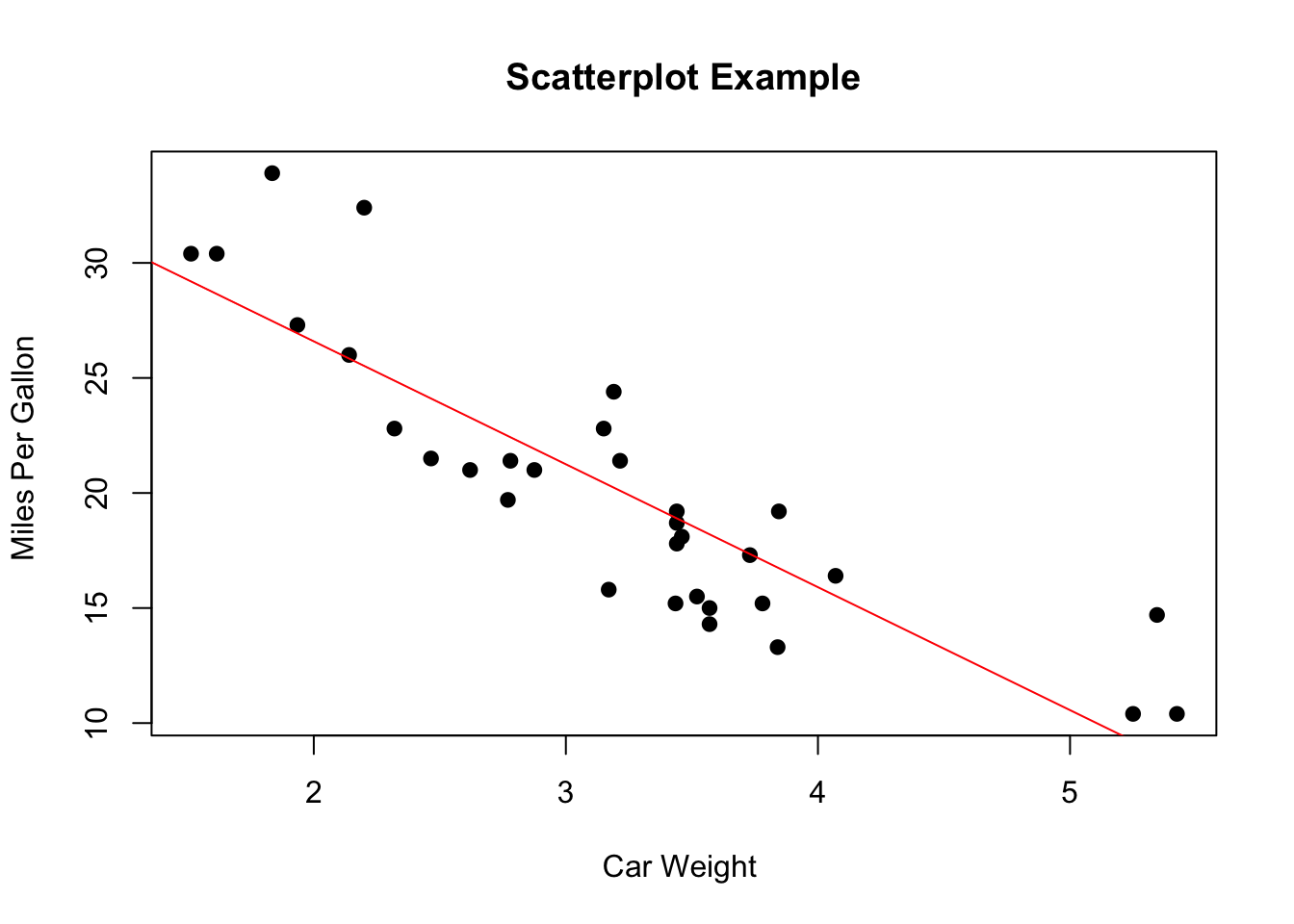
By using
scatterplot3dlibrary, we can plot a 3-dimensional scatterplot with 3 variables.rgllibrary can be helpful in visualizing 3-dimensional scatterplot interactively.
Code
# import scatterplot3d
library(scatterplot3d)

# plain 3D plot
scatterplot3d(mtcars$wt, mtcars$disp, mtcars$mpg, main = "3D Scatterplot")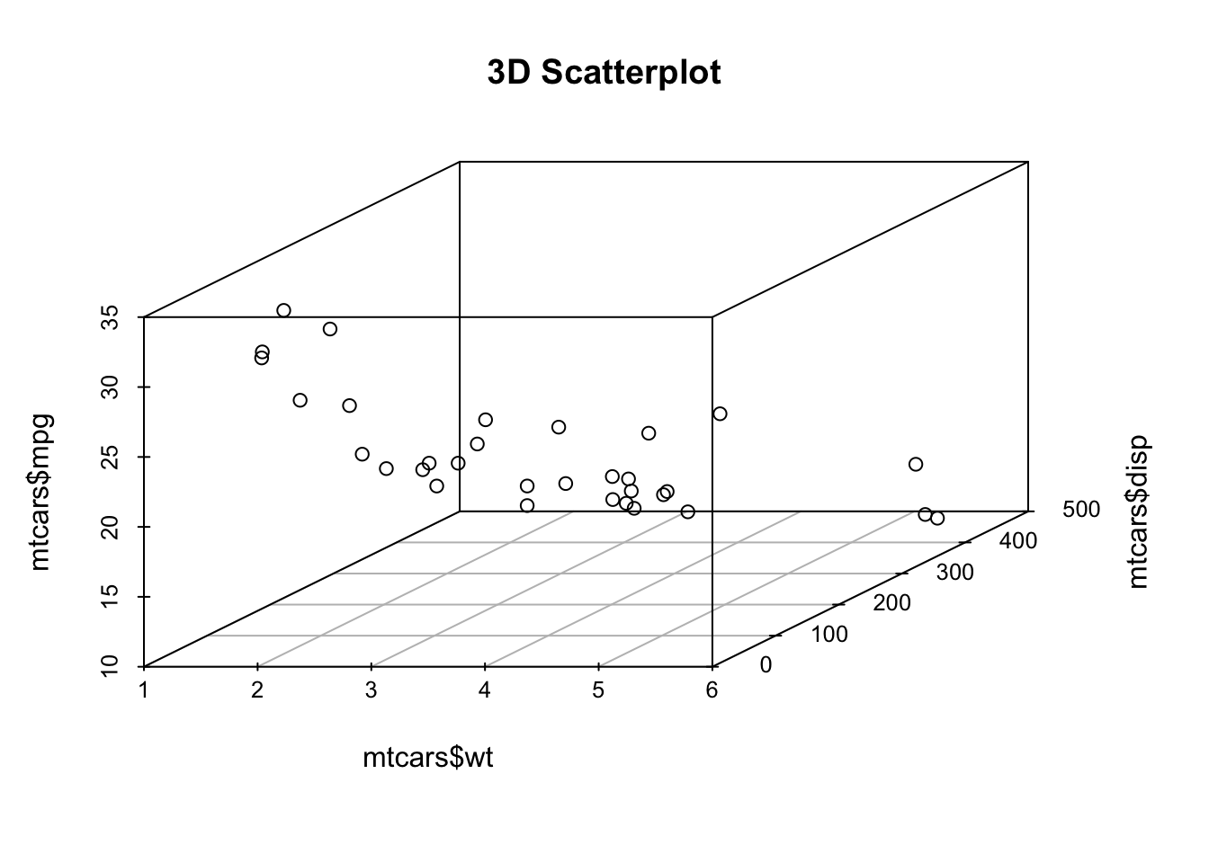
Code
# 3D plot with residuals
scatterplot3d(mtcars$wt, mtcars$disp, mtcars$mpg, pch = 16, highlight.3d = TRUE, type = "h", main = "3D Scatterplot",
    data = mtcars)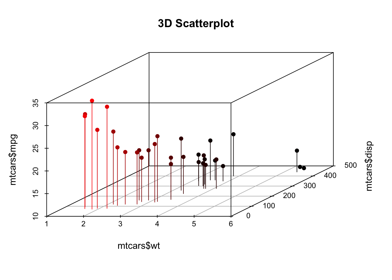
Code
# Spinning 3d Scatterplot
library(rgl)
plot3d(mtcars$wt, mtcars$disp, mtcars$mpg, col = "red", size = 3)
Useful source
1.11 Exercise & Quiz
1.11.1 Quiz: Exercise
- Use “Quiz-W1: Exercise” to submit your answers.
- Quiz forms are visible when you are currently logged into an NYU email account with Chrome browser due to privacy settings.
What do we mean when we say that this model does not constrain the predicted value to be a probability? It sure looks like a probability in this case. (link to exercise 1)
In (1) above, we give one way to understand/interpret “effects” (regression coefficients) in different ways. Do some of those ways sound more “causal” than others? Should any of them be? (link to exercise 2)
If we fit a
nullregression (no predictors; only a constant), what would the intercept tell us about the process for a Gaussian, logit, and Poisson link function? (link to Exercise 3)Is the likelihood \(L(\mu=0.5,\sigma^2=1|Y=1)\) bigger or smaller than \(L(\mu=1,\sigma^2=1|Y=1)\)? What does your intuition, looking at the formula, tell you? (link to Exercise 4)
1.11.2 Quiz: R Shiny
- Questions are from R shiny app “Lab 0: Method of Maximum Likelihood”.
- Use “Quiz-W1: R Shiny” to submit your answers.
[Maximum Likelihood Estimation: DGP]
- Naive model fit - Fit a linear model (
lm(y~x)ignoring heteroscadicity of errors. What variance (reported as residual standard error) do you expect?
[Maximum Likelihood Estimation the hard way]
- Evaluating the (log) likelihood - Test the function with the values that generated the data (DGP parameters). That call has been pre-loaded for you as well.
[Model Comparison]
- [Tab 3] Compare
lmtoglssolution - The method of generalized least squares allows for complex error structures through its weight and corr parameters. Use this function to reveal the proper s.e. for the heteroscedastic error model and compare to the priorlmfit (included in code).
[A Harder Model to fit]
- [Tab 4] Compute the MLE using
optim- Ask yourself why smaller samples contain less information about \(\phi\) and what might happen when \(\phi\) is incorrect
1.11.3 Quiz: Chapter
Use “Quiz-W1: Chapter” to submit your answers.
- What are NOT the example of “the limited dependent variables” ?
- What are the benefits of linear models?
- What are the conditions that is NOT need to be specified in a generalized linear modeling.
- What is the link function for Poisson distribution using ‘glm’ function in R?
- What is the purpose of the “Likelihood Ratio Test (LRT)” ?