Chapter 4 Chapter 4: Poisson Regression and Extensions
 ## Poisson Regression
4.0.1 Examples of count data
What type of outcomes are counts?
- Number of articles published by a Ph.D. candidate
- Number of children ever born
- Number of new HIV+ cases (incidence) in a regional area in the last year
- Number of juvenile delinquencies (unit of analysis is important and needs to be specified)
4.0.2 Characteristics and concepts
- Take values 0, 1, 2, 3, 4, … (non-negative integers)
- Often concentrated near zero (i.e., with “rare” events, we tend to observe lower numbers)
The conceptual model for count data consists of an underlying rate of occurrence.
- Rate: occurrences per unit time.
- The faster the rate, the higher the number of counts we would expect in a fixed time period.
- These are expectations or tendencies – not absolutes.
- Exposure: The longer the time period, the higher the expected number of counts (compared with a shorter time period) given the same rate of occurrence. Exposure can also refer to geographic area exposed to a treatment.
Examples:
- Rate: Rabbits produce more offspring per birth cycle than deer.
- Exposure (time): the number of electric cars purchased in a year tends to be larger than the number purchased in a month.
- Exposure (population): a city of 1,000,000 is likely to have more smokers than a city of 100,000.
Note: As alluded to, there is variability (uncertainty) in actual, observed counts. Two students with the same underlying rate of paper writing could produce different numbers of papers in the same time period. The uncertainty is quantified in the variance of the distribution used to model the counts.
4.0.3 Poisson distribution
We typically model count data as deriving from a Poisson distribution with parameter \(\lambda\), the rate of occurrence. The density for such a probability distribution function (pdf) is: \[ P(Y=y)=\frac{{{e}^{-\lambda }}{{\lambda }^{y}}}{y!} \] Where \(Y\) is the random variable, and \(y\) is the observed number of counts (in a given unit of time). \(P(Y=y)\) can be read as “the probability of observing \(y\) counts”.
We are implicitly assuming that \(Y\) is observed with common exposure (time or space), and the rate of occurrence is defined with respect to one unit of that exposure. One unit can be 100,000 people, as in the incidence of a disease per 100,000 people in the population.
4.0.4 Poisson distributions for different levels of \(\lambda\)
Code
lambdas <- c(0.5, 1, 2, 5)
par(mfrow = c(2, 2))
set.seed(2044)
for (i in seq_along(lambdas)) {
    barplot(dpois(0:10, lambdas[i]), ylab = "P(Y=y)", xlab = "counts (y)", space = 0, names.arg = 0:10)
    title(main = bquote(lambda ~ "=" ~ .(lambdas[i])))
}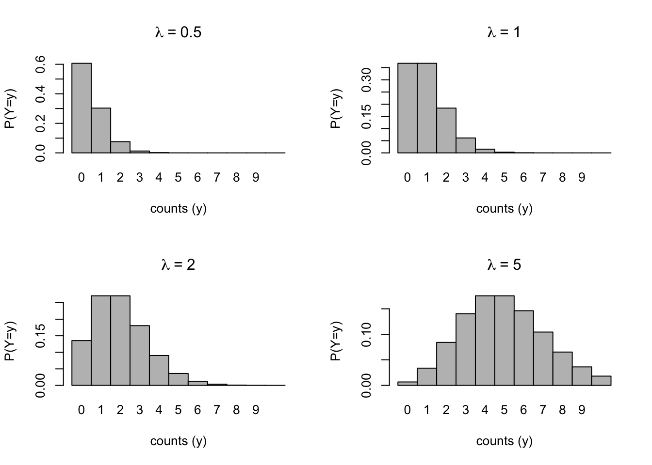
Notice how the expected count shifts to the right as \(\lambda\) increases. The distribution appears to be more normal, as well.
4.0.5 Rate of occurrence and mean count
An important feature of the Poisson distribution is that the parameter \(\lambda\) is the mean count. E(Y)= \(\lambda\). What’s interesting (and potentially problematic) about Poisson is that the variance of the count is also \(\lambda\).
Think about a sample of \(n\) subjects \(\{y_i\}_{i=1,\ldots,n}\), all of them with the same occurrence rate, \(\lambda\), but of course there is variability in outcomes. The average number of counts across people is a good estimate of the rate of occurrence. I.e., an estimate of the incidence rate is the number of new cases/total number exposed (e.g., to disease).
If the exposures \(n_i\) differ per person, we can take a weighted average: \[ \hat\lambda=\frac{1}{\sum_i n_i}\sum_i n_i\cdot y_i \]
And conversely the expected count for individual \(i\) is: \(n_i\lambda\), given exposure \(n_i\) (in units of time or space depending on the problem).
4.0.6 Poisson regression model
We can build a Poisson regression model that allows us to examine the relationship between predictors (explanatory variables) and the underlying rate of occurrence.1
The Poisson regression model is written: \[ \log\lambda_i=b_0 + b_1 X_{1i} + b_2 X_{2i} + \ldots + b_p X_{pi} \] Notice that the outcome \(Y_i\) is not specifically referenced, but it must be, so we additionally write \(Y_i\sim\mbox{Pois}(\lambda_i)\). We model differences in underlying rate \(\lambda_i\) via predictors represented by a matrix row \(X_i=\{X_{1i},X_{2i},\ldots,X_{pi}\}\).
4.0.7 Expressed as a GLM
The GLM components (for Poisson regression) are:
- \(Y_i \sim \mbox{Pois}(\lambda_i)\)
- \(\eta_i = X_i\beta\)
- \(g(\lambda_i) = \log(\lambda_i)=\eta_i\), thus \(\lambda_i=g^{-1}(\eta_i)=\exp(\eta_i)\).
4.0.8 Model types (review)
Where would ordinal regression go in this table? As a variant of multinomial, with a cumulative odds link.
4.0.9 Example: Articles Published
We use data from Long(1990) on the number of publications produced by Ph.D. Biochemists. There are the following variables in the dataset:
DSN: art.csv (CSV format)

art:        articles in last three years of Ph.D.
fem:        female=1, male=0
mar:        married=1, not married=0
kid5:       number of children under age six
phd:        prestige of Ph.D. program
ment: articles by mentor in three years- The outcome variable is the count/number of articles published in the last three years of Biochemistry PhD.
- The underlying rate of occurrence – the rate of publication with respect to exposure of three-year period that is common to all subjects – is what we wish to model.
- Potential Research Questions:
- What factors are related to the number of publications?
- Specific variables to consider: gender, marital status, having young kids and mentorship etc.
Code
articles <- read.csv("./Data/art.csv")
barplot(table(articles$art), main = "Observed Article Counts")
text(16, 200, paste0("mean=", round(mean(articles$art), 2), "\nvar=", round(var(articles$art), 2)), adj = 1)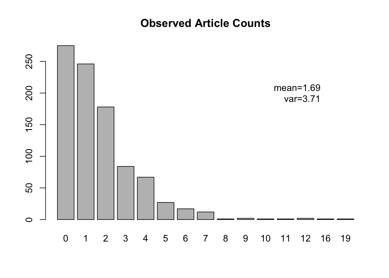
4.0.10 Unconditional model
First we fit a Poisson model without any predictors to understand how to interpret the intercept.
- Without predictors (\(X_i\)), the intercept is an estimate of \(\log\lambda\) across the entire data.
- In other words, we are assuming all subjects have same rate of occurrence.
- You can call this the marginal or unconditional rate as well.
Code
art.pois0 <- glm(art ~ 1, data = articles, family = poisson)
summary(art.pois0)
##
## Call:
## glm(formula = art ~ 1, family = poisson, data = articles)
##
## Deviance Residuals:
## Min 1Q Median 3Q Max
## -1.8401 -1.8401 -0.5770 0.2294 7.5677
##
## Coefficients:
## Estimate Std. Error z value Pr(>|z|)
## (Intercept) 0.52644 0.02541 20.72 <2e-16 ***
## ---
## Signif. codes: 0 '***' 0.001 '**' 0.01 '*' 0.05 '.' 0.1 ' ' 1
##
## (Dispersion parameter for poisson family taken to be 1)
##
## Null deviance: 1817.4 on 914 degrees of freedom
## Residual deviance: 1817.4 on 914 degrees of freedom
## AIC: 3487.1
##
## Number of Fisher Scoring iterations: 5A simple mathematical derivation shows that the estimate of \(\lambda\) is the same as the sample mean, which we showed in the barplot. If we exponentiate the estimate of the intercept to recover \(\hat\lambda\), we get 1.69.
4.0.11 Incorporating covariates
We will add all of the predictors available to a model for article count and fit a Poisson regression.
Code
art.pois1 <- glm(art ~ fem + mar + kid5 + phd + ment, data = articles, family = poisson)
summary(art.pois1)
##
## Call:
## glm(formula = art ~ fem + mar + kid5 + phd + ment, family = poisson,
## data = articles)
##
## Deviance Residuals:
## Min 1Q Median 3Q Max
## -3.5672 -1.5398 -0.3660 0.5722 5.4467
##
## Coefficients:
## Estimate Std. Error z value Pr(>|z|)
## (Intercept) 0.459860 0.093335 4.927 8.35e-07 ***
## femWomen -0.224594 0.054613 -4.112 3.92e-05 ***
## marSingle -0.155243 0.061374 -2.529 0.0114 *
## kid5 -0.184883 0.040127 -4.607 4.08e-06 ***
## phd 0.012823 0.026397 0.486 0.6271
## ment 0.025543 0.002006 12.733 < 2e-16 ***
## ---
## Signif. codes: 0 '***' 0.001 '**' 0.01 '*' 0.05 '.' 0.1 ' ' 1
##
## (Dispersion parameter for poisson family taken to be 1)
##
## Null deviance: 1817.4 on 914 degrees of freedom
## Residual deviance: 1634.4 on 909 degrees of freedom
## AIC: 3314.1
##
## Number of Fisher Scoring iterations: 5While we could interpret these effects in terms of the log-rate, it is more common to exponentiate these effects.
4.0.12 Relative incidence ratio/risk ratio interpretation
- The exponentiated effects transform the effects so that they are multiplicative in the rate
- Values greater than 1 indicate increased risk for the new value of the predictor.
- For a binary predictor, this relative risk ratio (or incidence ratio) is simply the new risk associated with being “TRUE” for the indicator as opposed to “FALSE.”
- Relative risk ratios are defined in certain contingency tables as well
- In this case, exposure to a toxin or treatment is evaluated as to whether there is an increased or decreased risk of a (negative or bad) outcome.
The same model fit, with exponentiated coefficients is given next:
Code
# jtools::summ(art.pois1,exp=T)

# ERROR MESSAGE ! Undefined control sequence. <recently read> \cellcolor
The model fit is described by:
- A \(\chi^2\) test on 5 degrees of freedom. This is a comparison of the null model deviance to this model’s deviance. The null model is the model with a single intercept and no predictors. This test of whether adding the predictors “improves” model fit; it is significant.
- The pseudo-\(R^2\) terms are attempts to quantify explained variance, but for the most part, they are not terribly informative.
- The effect associated with women is 0.80; interpreted multiplicatively, all else equal, women have on average \(20\%\) fewer publications.
- Having young children and being single also have effects under 1, suggesting fewer articles on average.
- The latter may be associated with a long-studied effect known as the “marriage premium.” That literature suggests that an interaction between sex and marriage might prove useful.
- Having a productive a mentor is associated with greater productivity, on average, all else equal.
- Importantly, the intercept term now is the log(\(\lambda\)) for the reference group (when \(X\) variables all take value 0, which may or may not be a realistic level).
4.0.13 Making predictions
Below, we make predictions for single women and men, varying the number of young children. The predictions are the expected count, which is not likely to be an integer.
Code
newdata <- data.frame(fem = rep(c("Women", "Men"), each = 4), mar = "Single", kid5 = rep(0:3, times = 2), phd = mean(articles$phd),
    ment = mean(articles$ment))
preds <- predict(art.pois1, newdata = newdata, type = "response")
cbind(newdata, preds)4.0.14 Pseudo-\(R^2\)
- Recall that we can make predictions for the given predictor patterns \(X_i\).
- These allow us to form residuals and assess fit.
- Recall that observed data will always be non-negative integers
- But predictions are based on the underlying rate, whose mean is not likely to be exactly an integer.
Code
preds <- predict(art.pois1, type = "response")
plot(preds, jitter(articles$art), pch = 16, cex = 0.9, xlab = "predicted", ylab = "observed", col = 2 + articles$kid5,
    xlim = c(0, 6), ylim = c(0, 8))
abline(a = 0, b = 1, col = 8)
points(0:6, 0:6, pch = 1, lwd = 2, col = 1)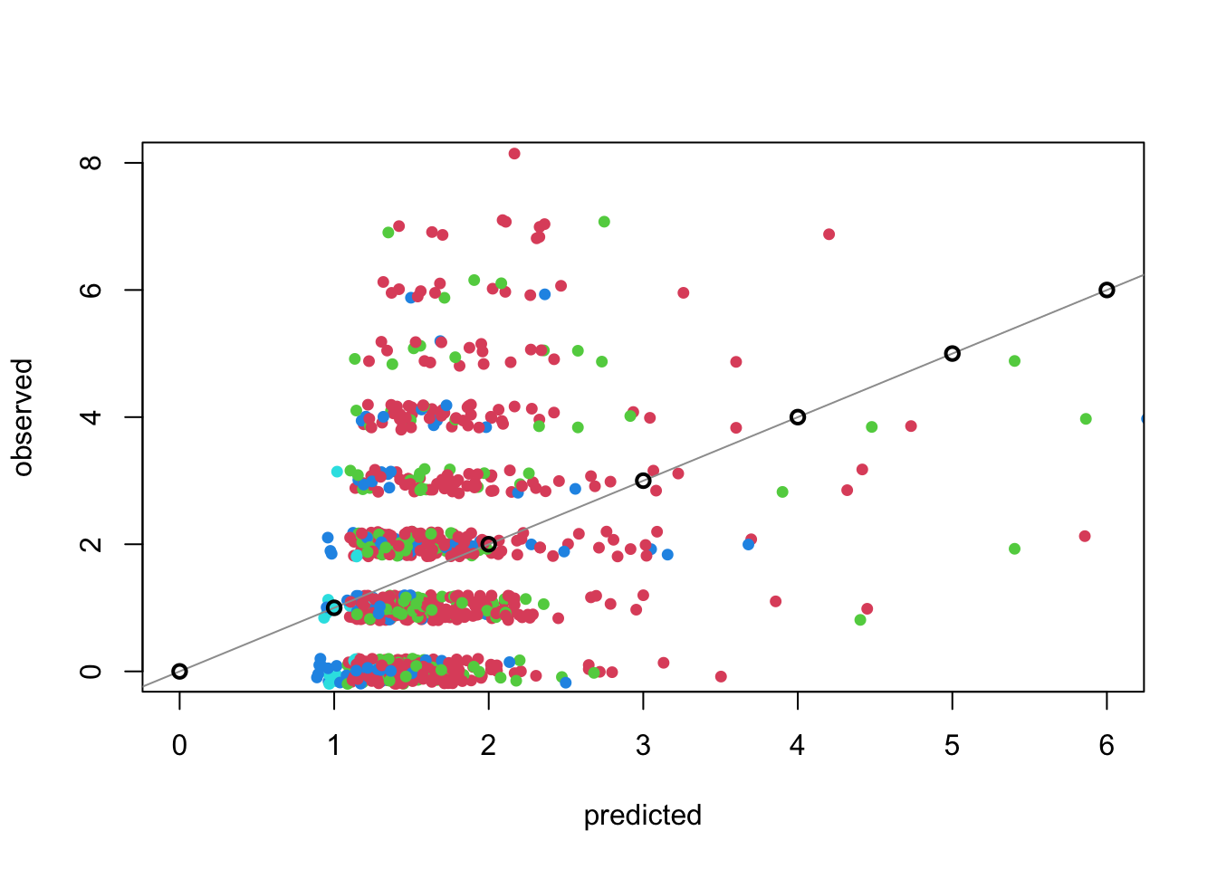
Notes:
- The line \(y=x\) would be perfect agreement, but this is misleading as we can only observe integer values.
- The large black circles indicate truly perfect, integer agreement. A nearly unattainable goal.
- The concentration of predictions between 1 and 2 suggests that we don’t have a lot of explanatory power. The observed span a much larger range.
What may be less apparent at first is that these predictions lend themselves to a “natural” \(R^2\)-like measure (such measures are called pseudo-\(R^2\)) that mimics the usual notion of proportion of variance explained. By computing residuals using observed and predicted values, we derive Efron’s pseudo-\(R^2\):
\[ R^2_{\mbox{Efron}}=1-\frac{\sum_i (y_i-\hat y_i)^2}{\sum_i (y_i-\bar y)^2} \]
Another attempt to describe fit is often attributed to McFadden and involves the ratio of the loglikelihoods of a given model to the null model:
\[
R^2_{\mbox{McFadden}}=1-\frac{LL_{\mbox{model}}}{LL_{\mbox{null}}}
\]
We provide R code to reproduce these two measures, one of which (McFadden’s) is given in the prior model summary using jtools::summ on a glm fit.
Code
efron <- 1 - var(articles$art - preds)/var(articles$art)
mcfadden <- as.numeric(1 - logLik(art.pois1)/logLik(art.pois0))
#
efron
## [1] 0.08807301Code
mcfadden## [1] 0.05251839We note that there is an R function in package Desctools that can produce a wide array of these measures. We also note that the Cragg-Uhler measure reported in the model summary is more commonly known as Nagelkerke’s. We generate all of these, below:
Code
DescTools::PseudoR2(art.pois1, which = "Efron")## Efron
## 0.08807301Code
DescTools::PseudoR2(art.pois1, which = "McFadden")## McFadden
## 0.05251839Code
DescTools::PseudoR2(art.pois1, which = "Nagelkerke")## Nagelkerke
## 0.185411These compare well with those that we manually constructed and with the model summary output.
4.0.15 Varying Exposure (example)
DSN: MASS::ships (Ship damage data in MASS package)

type:       coded 1-5 for A, B, C, D and E,
year:       year of construction: 1960-64, 1965-70, 1970-74, 1975-79
period:     period of operation (60=1960-74, 75=1975-79)
service:    months of service, ranging from 45 to 44882
incidents:  damage incidents, ranging from 0 to 58.
The outcome count variable is the number of damage incidences. The longer a ship is in service, the more damage we expect to see, even if the incidence rate per fixed period is the same.
We need to consider counts in the context of time of exposure. In this case, the rate \(\lambda\) and mean number of counts has the following relationship:
\[ E(Y)= \lambda\cdot T \] where \(T\) is exposure time, sometime called time at risk.
To fit a Poisson regression properly, we need to account for exposure time. In some ways, it looks like the only change to the specification of the GLM is in the DGP:
- \(Y_i \sim \mbox{Pois}(\lambda_i)\)
becomes
- \(Y_i \sim \mbox{Pois}(n_i\lambda_i)\)
where \(n_i\) is the exposure (\(T\) in the above formulation). Having an extra term in the DGP is fine, mathematically, but how would we specify the information contained in the exposures \(n_i\) into a model? It’s like a predictor, only it doesn’t quite follow the usual rules.
We note that given \(\log(\lambda_i)=X_i\beta\), add \(\log n_i\) to both sides of the equation, and then \[ \log(\lambda_i)+\log n_i=X_i\beta+\log n_i \] or \[ \log(n_i\lambda_i)=\log n_i+X_i\beta \]
- Thus adding an offset of \(\log n_i\) to the righthand equation models the log expected rate
- This is exactly of the same form as the DGP.
- There is no parameter being set - the coefficient on the offset is identically equal to one.
- Given the difference between the underlying rate and the expected counts with different exposures, we have to be careful that we’re actually modeling the expected count, which maps directly onto the observed counts.
Code
ships <- MASS::ships
ships <- ships %>%
    filter(service > 0)
ship.pois3 <- glm(incidents ~ type + factor(year) + factor(period) + offset(log(service)), data = ships, family = poisson)
# jtools::summ(ship.pois3)- This model has such a high pseudo-\(R^2\) that we are worried, and decide to examine the fit through a plot of predictions vs. observed:
Code
preds <- predict(ship.pois3, type = "response")
plot(preds, jitter(ships$incidents), pch = 16, cex = 0.9, xlab = "predicted", ylab = "observed", col = factor(ships$year),
    xlim = c(0, 60), ylim = c(0, 60))
abline(a = 0, b = 1, col = 8)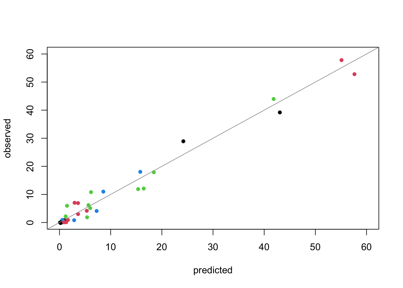
Evidence of excellent fit.
4.0.16 Residuals
While the sample is small, we should examine residuals, looking for outliers or other violations of model assumptions.
Code
res <- residuals(ship.pois3, type = "deviance")
sm::sm.density(res, model = "normal")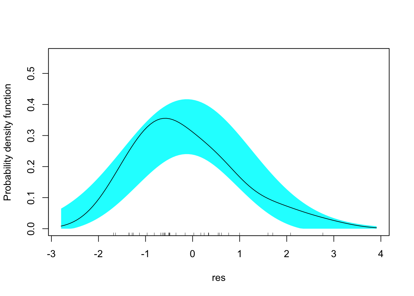
A core assumption of Poisson regression is that the mean equals the variance of the outcome, conditional on predictors (covariate pattern). We cannot check this for every covariate pattern, of course, but we certainly can test it in the raw outcome. However, even if the raw outcome is highly divergent from a Poisson distribution, it is still possible for the conditional distribution to be Poisson. So we need methods for testing for this, or modeling it directly.
Let us examine it for the original outcome in the shipping data:
Code
plot(density(ships$incidents), main = "Ships: incidents", ylim = c(0, 0.12))
lines(density(rpois(1000, lambda = mean(ships$incidents))), col = 5)
legend("topright", col = c(1, 5), lty = c(1, 1), legend = c("Original", "Poisson-matched"), bty = "n")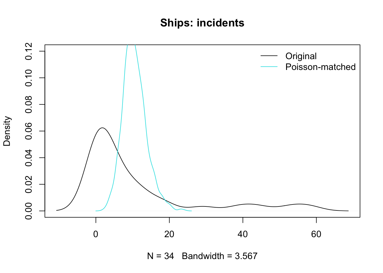
- You can see from this plot that it is implausible that the original data were Poisson
- But the model seems to make good predictions
- Maybe conditionally, the outcomes are Poisson (with rates that vary based on the model/conditioning).
4.0.17 Issue of Overdispersion in GLM
Note: there are many reasons that a model doesn’t fit the data well:
- Omitted explanatory variables
- Unobserved heterogeneity
- Wrong functional form (linear/nonlinear, interaction, etc.)
- Outliers, overly influential points, etc.
In GLM, model misfits often induce over-dispersion: the variance is greater than what the model predicts.
4.0.18 Relationship between mean and variance in some GLMs
Up to this point, we have not emphasized this, but the relationship between the mean and variance is an important component of a GLM. We did not need to worry about it because the choice of distribution in the DGP determined the mean/variance relationship.
- In the normal distribution, the mean \((\mu=X\beta)\) and variance \(\sigma^2\) are two separate parameters, estimated separately. There is no dependence between them in a normal distribution. Thus, overdispersion is not an issue.
- If the mean of a Poisson is \(\lambda\), then the variance is also \(\lambda\). When we model \(\log(\lambda)=X\beta\), we assume the relationship of equality between mean and variance holds.
- If the mean of a binomial proportion is \(p\), the variance is \(p(1-p)/n\), assuming \(n\) draws. When we model \(\mbox{logit}(p)=X\beta\), we assume that the variance \(p(1-p)/n\) is determined accordingly.
- If the variance doesn’t behave as the mean structure suggests for that distribution, then we have a problem with overdispersion (or occasionally, underdispersion).
4.0.19 Forms of Over-dispersion in Poisson and Binomial models
- Dispersion up to a constant term: A simple situation when the true variance is proportional to what the model predicts.
- For Poisson model: \(\mbox{var}(Y)=\theta\lambda,\ \theta>1\)
- For Binomial model: \(\mbox{var}(Y)=\theta p(1-p)/n,\ \theta>1\)
- : In the classic GLM setup, we assume that the parameter of interest for each individual is completely determined by the (X\(\beta\)) part. But often there is unexplained individual heterogeneity.
- For count data, when the rate of occurrence of each individual is \(\nu_i\lambda\), where \(\nu_i\) is the individual factor following a gamma distribution, the distribution of the counts will be Negative Binomial (NB) distribution (if NB mean is \(\lambda\), NB variance is greater than \(\lambda\)).
- For grouped binomial data, we can multiply the probability of an outcome by a group-specific scaling factor. This is beyond the scope of the course.
- Structural zeros: some subjects are not subject to any risk. E.g., number of cigarettes smoked per day among the non-smokers. The probability of having outcomes greater than 0 for non-smokers is 0, but it could follow a Poisson for smokers.
All the above situations will lead to a problem of over-dispersion. The overdispersion problem in the Poisson model is much easier to handle than in Binomial model.
4.0.20 Implications and Diagnosis of Over-dispersion
A direct implication of over-dispersion is that the standard error of the regression coefficients are wrong, hence the statistical inferences will be incorrect.
The interpretation of the model is also different when there is unobserved heterogeneity or structural zeros.
- We can use deviance residual to check for any evidence of overdispersion.
- Under the hypothesis that the model fits the data, the sum of squared deviance residuals has a Chi-square distribution with degree freedom of \(n-p\).
- The mean of a \(\chi^2_{n-p}\) distributed random variable is \(n-p\).
- So for a well fitting model, we expect the average squared Deviance residual to be \(n-p\).
- When the average squared Deviance residual is greater than \(n-p\), it suggests that the model doesn’t fit the data very well.
- Of course, we can do a statistical test.
4.0.21 R’s glm function and over dispersion.
R does not provide an estimate of dispersion in the glm function, but it is easy enough to compute. We build a function to do so.
- The sum of squared deviance residuals are distributed as \(\chi^2_{d}\), where \(d\) is the residual degrees of freedom.
- The sum is often called the deviance
- Roughly speaking, the ratio of the deviance to the residual degrees of freedom measures V(Y)/E(Y) [net of predictors].
- If this value is close to 1, then we don’t have an overdispersion problem.
- If they are much greater than 1, then we have an overdispersion problem.
- Sometimes there can be a underdispersion problem, where the scale parameter is much smaller than 1. It is a rare situation.
Code
glm.disp <- function(x) {
    dev.res <- residuals(x, type = "deviance")
    disp.est <- sum(dev.res^2)  #this is chi-sq w/ df from the model
    df <- df.residual(x)  #use built-in function
    list(dispersion = disp.est/df, p = 1 - pchisq(disp.est, df))
}
print(rslt <- glm.disp(ship.pois3), digits = 3)
## $dispersion
## [1] 1.55
##
## $p
## [1] 0.0395- The dispersion is greater than one with this model
- More importantly, the statistical test suggests some residual overdispersion.
- This is in contrast to the visual inspection of the residuals we did earlier, which did not reveal deviation from normality.
- One quick fix to the over-dispersion problem is to scale up the standard errors proportionally based on the estimate of the dispersion.
- In this case, we would multiply all of the listed s.e. for the predictor effects by the square root of
disp.est=1.55. - This is likely to change the significance of your effects.
- In this case, we would multiply all of the listed s.e. for the predictor effects by the square root of
4.0.22 Quasi-Poisson model
There is a way to allow for overdispersion directly in the model, and we have already sketched the details. We make this a bit more formal:
For the quasi-Poisson model, very generally,
- \(E(Y) = \lambda\)
- \(V(Y) = \theta\lambda\) (not \(\lambda\) as in a regular Poisson model)
The model is fit using a quasi-likelihood, rather than a likelihood, which allows for and estimates this overdispersion parameter.
In R, this model is implemented by choosing quasipoisson as the family. We examine our original “full” model using the quasi-Poisson fit:
Code
ship.qpois3 <- glm(incidents ~ type + factor(year) + factor(period) + offset(log(service)), data = ships, family = quasipoisson)
summary(ship.qpois3)
##
## Call:
## glm(formula = incidents ~ type + factor(year) + factor(period) +
## offset(log(service)), family = quasipoisson, data = ships)
##
## Deviance Residuals:
## Min 1Q Median 3Q Max
## -1.6768 -0.8293 -0.4370 0.5058 2.7912
##
## Coefficients:
## Estimate Std. Error t value Pr(>|t|)
## (Intercept) -6.40590 0.28276 -22.655 < 2e-16 ***
## typeB -0.54334 0.23094 -2.353 0.02681 *
## typeC -0.68740 0.42789 -1.607 0.12072
## typeD -0.07596 0.37787 -0.201 0.84230
## typeE 0.32558 0.30674 1.061 0.29864
## factor(year)65 0.69714 0.19459 3.583 0.00143 **
## factor(year)70 0.81843 0.22077 3.707 0.00105 **
## factor(year)75 0.45343 0.30321 1.495 0.14733
## factor(period)75 0.38447 0.15380 2.500 0.01935 *
## ---
## Signif. codes: 0 '***' 0.001 '**' 0.01 '*' 0.05 '.' 0.1 ' ' 1
##
## (Dispersion parameter for quasipoisson family taken to be 1.691028)
##
## Null deviance: 146.328 on 33 degrees of freedom
## Residual deviance: 38.695 on 25 degrees of freedom
## AIC: NA
##
## Number of Fisher Scoring iterations: 5The estimated dispersion parameter \(\theta=\) 1.691 is a bit different from the one that we constructed “post hoc” (after fitting the model).
4.1 The Negative Binomial model
4.1.1 A model for overdispersion
A more sophisticated way to deal with over-dispersion is to take the individual heterogeneity into account and use negative binomial distribution to model the counts. This has been sketched, above.
Details: let’s assume that on average, the rate of occurrence for all the student in the sample is \(\lambda\). But we allow each individual to have a different rate of occurrence that is \(\nu_i\lambda\), where \(\nu_i\) is the individual factor.2
- Assume \(\nu_i\sim \mbox{Gamma}(\theta)/\theta\). This implies that \(E(\nu_i)=1\).
- To allow for individual-specific rates, \(Y_i\sim\mbox{Pois}(\nu_i\lambda_i)\).
- Then, \(E(Y_i)=\lambda_i\), but \(V(Y_i)=\lambda+\lambda^2/\theta=\lambda(1+\lambda/\theta)\).
The variance expression can be seen as a multiple, greater than one, of the original \(\lambda\).
The above defines a negative binomial distribution for counts \(Y\), with mean parameter \(\lambda\) and dispersion parameter \(\theta\).3
4.1.2 Simulating a Negative Binomial from its components
Let \(\theta=1\) and \(\lambda=3\). We expect a Poisson to have variance 3, but a negative binomial to have variance 12.
- First we generate the rescaled Gamma.
Code
set.seed(2044)
N <- 10000
theta <- 1
nu_i <- rgamma(N, theta)/theta
sm::sm.density(nu_i)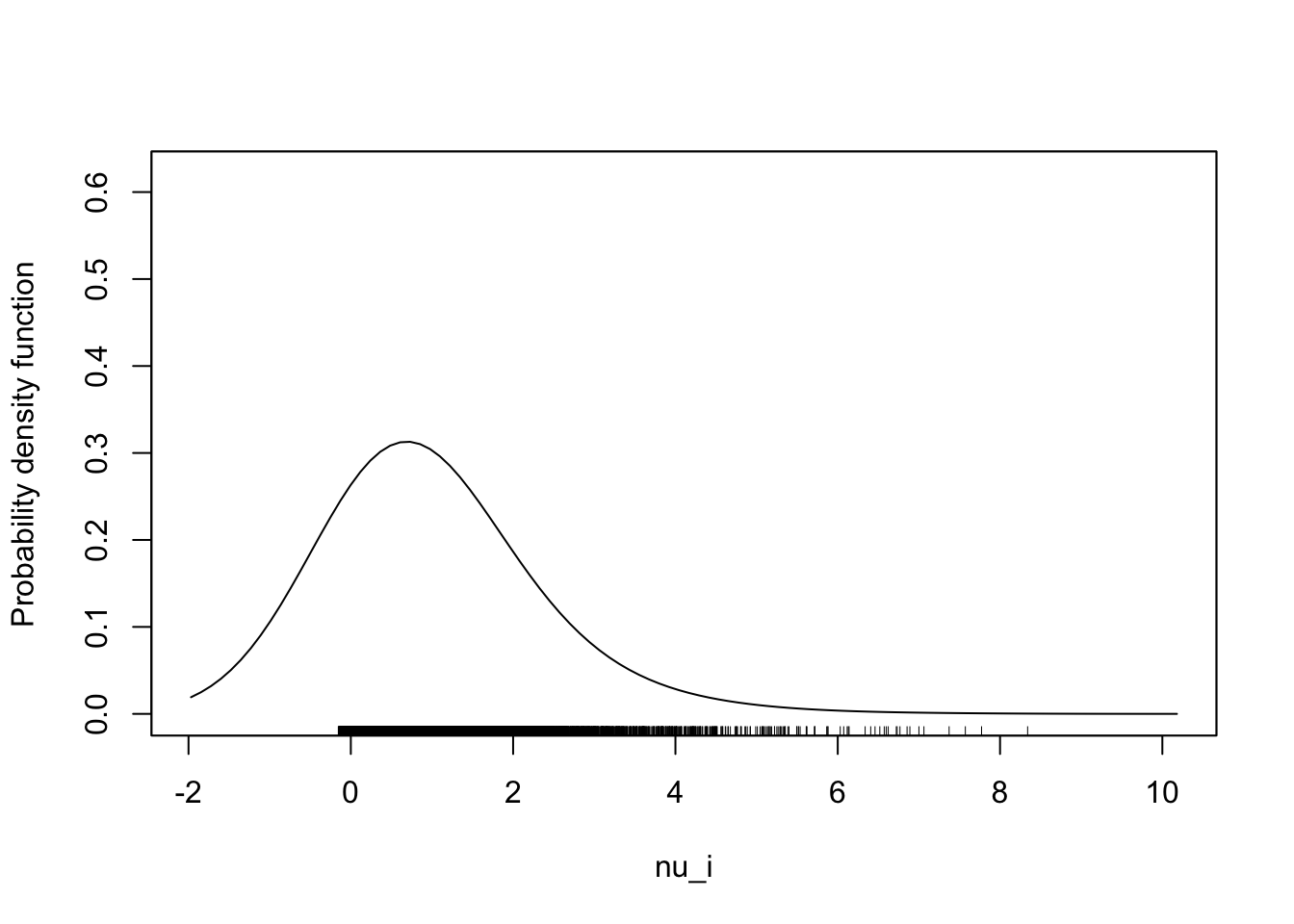
- Then we generate a Poisson, using a different rate parameter for every draw, based on the Gamma value drawn (\(\nu_i\)).
- This will inflate the variance of the Poisson
- You can think of it as jittering the underlying parameters to be a bit higher or lower, thereby extending the mass of the realized distribution to the left and right.
- The unadjusted Poisson with \(\lambda=3\) is the reference line.
Code
set.seed(2044)
N <- 10000
lambda <- 3
pois.sims <- rpois(N, nu_i * lambda)
tbl <- prop.table(table(pois.sims))

barplot(tbl, ylab = "P(Y=y)", xlab = "counts (y)", space = 0, ylim = c(0, 0.225))
title(main = bquote(lambda ~ "=" ~ .(lambda) ~ ";" ~ theta ~ "=" ~ .(theta)))
lines(density(rpois(N, lambda), bw = 1), col = 2, lwd = 3)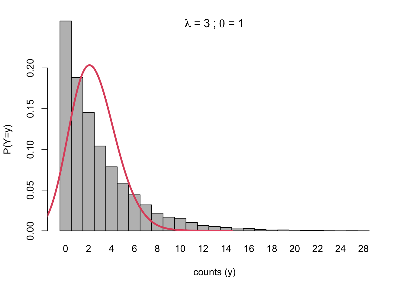
4.1.3 Negative Binomial Regression in R
- We fit the least complicated model first, and then add predictors.
- The model with a constant provides a simple test of overdispersion in the count distribution.
- The extent to which the theta parameter in this model is significant (we will use a likelihood ratio test against a non-inflated Poisson model) performs the test.
- We will use the
Rpackagepscland functionodTest.
Code
ship.nb0 <- MASS::glm.nb(incidents ~ 1 + offset(log(service)), data = ships)
summary(ship.nb0)
##
## Call:
## MASS::glm.nb(formula = incidents ~ 1 + offset(log(service)),
## data = ships, init.theta = 2.923204332, link = log)
##
## Deviance Residuals:
## Min 1Q Median 3Q Max
## -1.9194 -0.9286 -0.5283 0.3488 2.4190
##
## Coefficients:
## Estimate Std. Error z value Pr(>|z|)
## (Intercept) -5.7181 0.1377 -41.53 <2e-16 ***
## ---
## Signif. codes: 0 '***' 0.001 '**' 0.01 '*' 0.05 '.' 0.1 ' ' 1
##
## (Dispersion parameter for Negative Binomial(2.9232) family taken to be 1)
##
## Null deviance: 35.809 on 33 degrees of freedom
## Residual deviance: 35.809 on 33 degrees of freedom
## AIC: 173.38
##
## Number of Fisher Scoring iterations: 1
##
##
## Theta: 2.92
## Std. Err.: 1.21
##
## 2 x log-likelihood: -169.378Code
pscl::odTest(ship.nb0)## Likelihood ratio test of H0: Poisson, as restricted NB model:
## n.b., the distribution of the test-statistic under H0 is non-standard
## e.g., see help(odTest) for details/references
##
## Critical value of test statistic at the alpha= 0.05 level: 2.7055
## Chi-Square Test Statistic = 74.817 p-value = < 2.2e-16- The overdispersion is close to 3, and it’s deemed highly significant.
- We will add a single predictor next, then redo the test.
Code
ship.nb1 <- MASS::glm.nb(incidents ~ type + offset(log(service)), data = ships)
summary(ship.nb1)
##
## Call:
## MASS::glm.nb(formula = incidents ~ type + offset(log(service)),
## data = ships, init.theta = 7.617318123, link = log)
##
## Deviance Residuals:
## Min 1Q Median 3Q Max
## -1.9938 -0.9122 -0.3955 0.4986 2.3008
##
## Coefficients:
## Estimate Std. Error z value Pr(>|z|)
## (Intercept) -5.4847 0.2295 -23.902 <2e-16 ***
## typeB -0.6909 0.2760 -2.503 0.0123 *
## typeC -0.7169 0.3947 -1.816 0.0693 .
## typeD -0.1018 0.3834 -0.266 0.7905
## typeE 0.4582 0.3358 1.364 0.1725
## ---
## Signif. codes: 0 '***' 0.001 '**' 0.01 '*' 0.05 '.' 0.1 ' ' 1
##
## (Dispersion parameter for Negative Binomial(7.6173) family taken to be 1)
##
## Null deviance: 55.414 on 33 degrees of freedom
## Residual deviance: 36.612 on 29 degrees of freedom
## AIC: 167.6
##
## Number of Fisher Scoring iterations: 1
##
##
## Theta: 7.62
## Std. Err.: 4.00
##
## 2 x log-likelihood: -155.603Code
pscl::odTest(ship.nb1)## Likelihood ratio test of H0: Poisson, as restricted NB model:
## n.b., the distribution of the test-statistic under H0 is non-standard
## e.g., see help(odTest) for details/references
##
## Critical value of test statistic at the alpha= 0.05 level: 2.7055
## Chi-Square Test Statistic = 33.1525 p-value = 4.26e-09The estimated dispersion parameter \(\theta=\) 7.617, and it’s significant. We will add another predictor, then redo the test.
Code
ship.nb2 <- MASS::glm.nb(incidents ~ type + factor(year) + offset(log(service)), data = ships)
summary(ship.nb2)
##
## Call:
## MASS::glm.nb(formula = incidents ~ type + factor(year) + offset(log(service)),
## data = ships, init.theta = 27.11762495, link = log)
##
## Deviance Residuals:
## Min 1Q Median 3Q Max
## -1.7846 -1.0200 -0.4841 0.5163 2.1730
##
## Coefficients:
## Estimate Std. Error z value Pr(>|z|)
## (Intercept) -6.22349 0.27545 -22.594 < 2e-16 ***
## typeB -0.54201 0.21790 -2.487 0.0129 *
## typeC -0.65626 0.35287 -1.860 0.0629 .
## typeD -0.06245 0.32464 -0.192 0.8475
## typeE 0.35748 0.27166 1.316 0.1882
## factor(year)65 0.71392 0.22623 3.156 0.0016 **
## factor(year)70 0.90116 0.23031 3.913 9.13e-05 ***
## factor(year)75 0.62721 0.28432 2.206 0.0274 *
## ---
## Signif. codes: 0 '***' 0.001 '**' 0.01 '*' 0.05 '.' 0.1 ' ' 1
##
## (Dispersion parameter for Negative Binomial(27.1176) family taken to be 1)
##
## Null deviance: 86.760 on 33 degrees of freedom
## Residual deviance: 38.285 on 26 degrees of freedom
## AIC: 163.17
##
## Number of Fisher Scoring iterations: 1
##
##
## Theta: 27.1
## Std. Err.: 28.4
##
## 2 x log-likelihood: -145.165Code
pscl::odTest(ship.nb2)## Likelihood ratio test of H0: Poisson, as restricted NB model:
## n.b., the distribution of the test-statistic under H0 is non-standard
## e.g., see help(odTest) for details/references
##
## Critical value of test statistic at the alpha= 0.05 level: 2.7055
## Chi-Square Test Statistic = 2.0562 p-value = 0.07579- The estimated dispersion parameter \(\theta=\) 27.118
- But the LTR deems it not significant.
- We will add the last predictor, then redo the test.
Code
ship.nb3 <- MASS::glm.nb(incidents ~ type + factor(year) + factor(period) + offset(log(service)), data = ships)
summary(ship.nb3)
##
## Call:
## MASS::glm.nb(formula = incidents ~ type + factor(year) + factor(period) +
## offset(log(service)), data = ships, init.theta = 52549.56866,
## link = log)
##
## Deviance Residuals:
## Min 1Q Median 3Q Max
## -1.6768 -0.8293 -0.4370 0.5058 2.7911
##
## Coefficients:
## Estimate Std. Error z value Pr(>|z|)
## (Intercept) -6.40589 0.21749 -29.454 < 2e-16 ***
## typeB -0.54335 0.17762 -3.059 0.00222 **
## typeC -0.68738 0.32906 -2.089 0.03672 *
## typeD -0.07596 0.29060 -0.261 0.79379
## typeE 0.32562 0.23590 1.380 0.16750
## factor(year)65 0.69714 0.14970 4.657 3.21e-06 ***
## factor(year)70 0.81840 0.16982 4.819 1.44e-06 ***
## factor(year)75 0.45339 0.23321 1.944 0.05188 .
## factor(period)75 0.38448 0.11831 3.250 0.00116 **
## ---
## Signif. codes: 0 '***' 0.001 '**' 0.01 '*' 0.05 '.' 0.1 ' ' 1
##
## (Dispersion parameter for Negative Binomial(52549.57) family taken to be 1)
##
## Null deviance: 146.247 on 33 degrees of freedom
## Residual deviance: 38.691 on 25 degrees of freedom
## AIC: 156.56
##
## Number of Fisher Scoring iterations: 1
##
##
## Theta: 52550
## Std. Err.: 566024
## Warning while fitting theta: iteration limit reached
##
## 2 x log-likelihood: -136.564Code
pscl::odTest(ship.nb3)## Likelihood ratio test of H0: Poisson, as restricted NB model:
## n.b., the distribution of the test-statistic under H0 is non-standard
## e.g., see help(odTest) for details/references
##
## Critical value of test statistic at the alpha= 0.05 level: 2.7055
## Chi-Square Test Statistic = -0.0026 p-value = 0.5- The overdispersion parameter is very large.
- We note that \(\frac{1}{\theta}\) is thus near 0, eliminating the overdispersion.
- I would revert to the quasi-Poisson model at this point, consider large theta to mean overdispersion goes away with these controls, or use alternative software.
4.1.4 Comparison of Poisson and NB predictions
- We return to the second model, with only one predictor, because it demonstrates clear overdispersion.
- The value of the mean, \(\lambda\) varies depending on the predictor,
typeand exposure time. - We note that these place it in the range 10-30, approximately.
- So the impact of overdispersion parameter \(\theta=\) 7.617 can be substantial.
- In practice this translates to a wider range of predictions from a NB model, as compared to a Poisson model.
- We can see this from this plot after making predictions for Poisson and NB models:
Code
ship.pois1 <- glm(incidents ~ type + offset(log(service)), data = ships)
pred.nb1 <- pred.pois1 <- predict(ship.pois1, type = "response")
actual <- dff <- data.frame(actual = ships$incidents, pred = predict(ship.nb1, type = "response"), model = 1)
dff <- rbind(dff, data.frame(actual = ships$incidents, pred = predict(ship.pois1, type = "response"), model = 2))

ggplot(data = dff, aes(x = actual, y = pred, color = factor(model, labels = c("Negative-Binomial", "Poisson")))) +
    geom_point() + ylab("Predicted") + xlab("Actual") + theme(legend.title = element_blank()) + geom_abline(intercept = 0,
    slope = 1)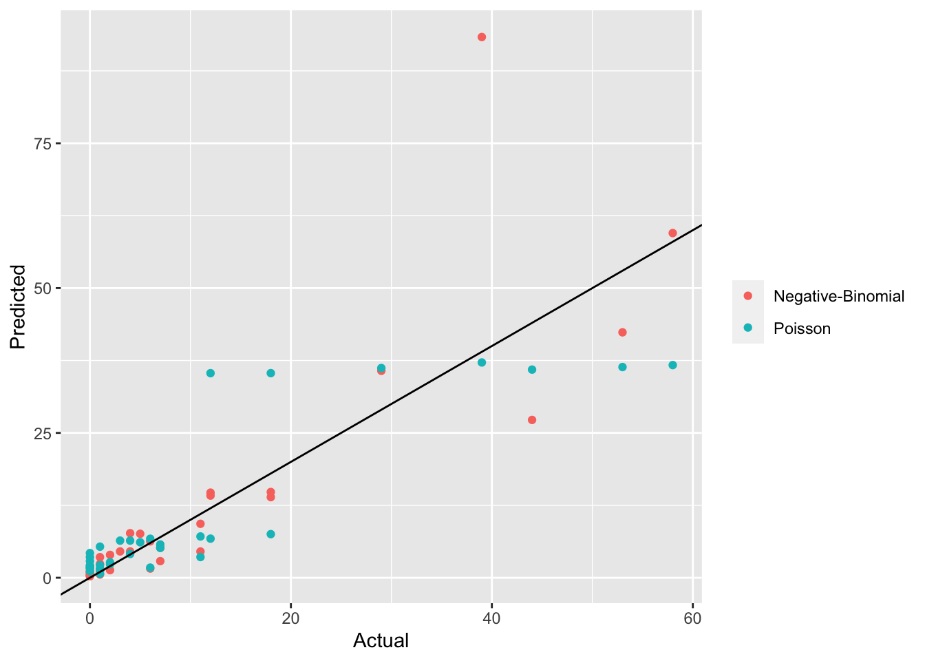
- The NB model seems to make better predictions particularly for larger actual counts.
4.2 Zero-inflated Poisson model
4.2.1 Another overdispersion model
- Another form of overdispersion occurs when there are “excess zeros.”
- The Zero-inflated Poisson model was created to handle this case.
- The basic idea is that some individuals in the study either cannot or do not intend to ever participate in the activity being studied.
4.2.2 Examples of Zero-Inflation
- An example is smoking or drinking: a study the adult population as a whole is likely to reveal that some people “never smoke” or “never drink.”
- The count of how many cigarettes or drinks consumed daily will be zero for these individuals, inflating the zero count beyond what would be expected in a Poisson distribution.
- The mean of this distribution is influenced by these zeros, so the non-zero observations will appear overdispersed, as compared to that mean.
- The count of how many cigarettes or drinks consumed daily will be zero for these individuals, inflating the zero count beyond what would be expected in a Poisson distribution.
- As another example, in our study of a population of Ph.D. students, suppose that some have decided to go to industry after graduation so they do not have any plans of writing any articles in graduate school. There are actually two populations:
- Group 1: students have no intention to publish at all. The number of publications is 0 among this group.
- Group 2: students have intention to publish.
- Their number of articles published follow a Poisson distribution.
- Some of them may still have 0 publications at the time of study, consistent with a Poisson distribution, but in this case, the zeros are not “excessive.”
4.2.3 ZIP model mathematical representation
There is some type of “choice” model that predicts whether or not the individual is in group 0 or 1. In group 0, their outcome is 0; in group 1, it follows a Poisson regression. We will write this first model in R notation.
The model for group assignment \(Z\): glm(Z~W,family='logit') where \(W\) are predictors of that membership.
- When \(Z_i=0\), \(Y_i=0\)
- When \(Z_i=1\), \(Y_i\sim\mbox{Pois}(\lambda_i)\), with \(\log\lambda=X_i\beta\), the core of a Poisson regression model.
4.2.4 ZIP model Simulation
We will simulate data from a simple ZIP model for which the probability of a deterministic zero is 25% and then the remaining 75% of the population follows a Poisson with rate parameter \(\lambda=3\).
Code
set.seed(2044)
N <- 10000
Z <- rbinom(N, 1, p = 0.75)
n.nonuser <- sum(Z == 0)
Z <- factor(Z, levels = 0:1, labels = c("non-user", "user"))
Y <- rep(0, N)  # outcome default to zero (for non-user)
Y[Z == "user"] <- rpois(N - n.nonuser, 3)  #the sample size here is based on the first logit model
tbl <- table(Y)
barplot(tbl, main = "Distribution: Simulated ZIP")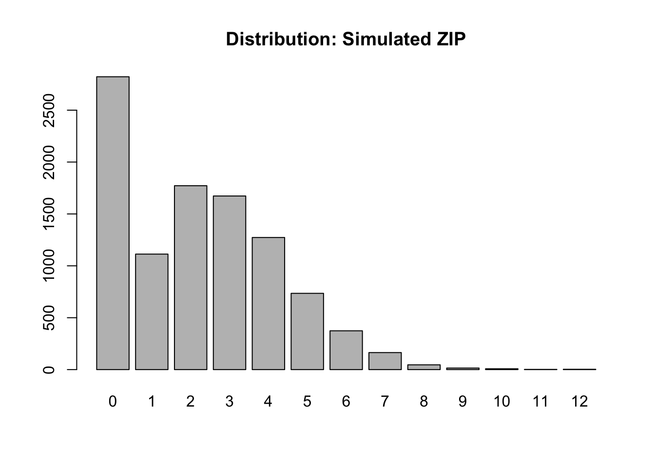
Code
# now break it into components
X <- as.numeric(names(tbl))
len <- length(X)
counts.all <- as.numeric(tbl)
counts.nonuser <- c(n.nonuser, rep(0, len - 1))
counts.user <- counts.all - counts.nonuser
df <- data.frame(type = c(rep("non user", len), rep("user", len)), count = c(counts.nonuser, counts.user), X = rep(X,
    times = 2))
ggplot(df, aes(fill = type, y = count, x = X)) + geom_bar(position = "stack", stat = "identity") + xlab("")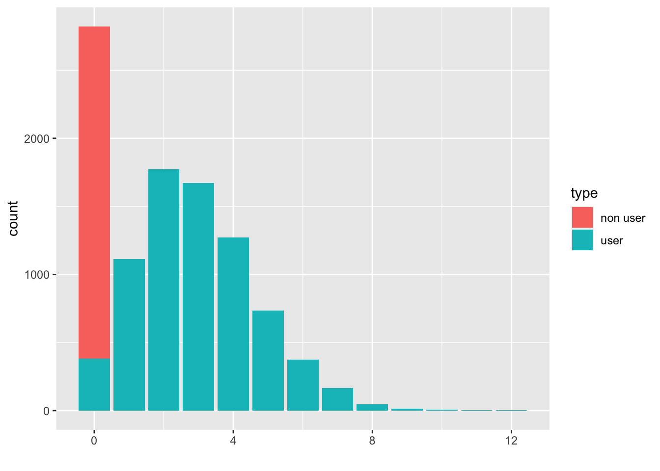
- The outcome (count) \(Y\) is constructed in two phases, as indicated by the DGP sketched previously.
- The first plot is just the distribution of the mixture of users and non-users.
- The second takes a bit more coding, but reveals in red the subgroup of non-users that contribute to the zero inflation.
- The mean and variance of a Poisson is the same, and in this case, would be 3 were it not for the zero inflation.
- With zero inflation, the mean shrinks to 2.25 and the variance is 3.86, which is disproportionately larger than the mean.
4.2.5 ZIP models in R
Returning to the paper publication data.
Zip model can be fit using the zeroinfl function in pscl package.
Code
art.zip1 <- pscl::zeroinfl(art ~ fem + mar + kid5 + phd + ment | 1, data = articles, family = poisson)
summary(art.zip1)
##
## Call:
## pscl::zeroinfl(formula = art ~ fem + mar + kid5 + phd + ment | 1, data = articles, family = poisson)
##
## Pearson residuals:
## Min 1Q Median 3Q Max
## -1.5296 -0.9976 -0.3026 0.5398 7.2884
##
## Count model coefficients (poisson with log link):
## Estimate Std. Error z value Pr(>|z|)
## (Intercept) 0.685967 0.103522 6.626 3.44e-11 ***
## femWomen -0.231609 0.058670 -3.948 7.89e-05 ***
## marSingle -0.131972 0.066130 -1.996 0.046 *
## kid5 -0.170474 0.043296 -3.937 8.24e-05 ***
## phd 0.002526 0.028511 0.089 0.929
## ment 0.021543 0.002160 9.973 < 2e-16 ***
##
## Zero-inflation model coefficients (binomial with logit link):
## Estimate Std. Error z value Pr(>|z|)
## (Intercept) -1.6813 0.1558 -10.79 <2e-16 ***
## ---
## Signif. codes: 0 '***' 0.001 '**' 0.01 '*' 0.05 '.' 0.1 ' ' 1
##
## Number of iterations in BFGS optimization: 13
## Log-likelihood: -1621 on 7 Df- It is useful to examine the estimate from the model that predicts use, which in this instance has no predictors, but a constant of -1.68
- Applying the inverse logit or expit function, this is 0.16.
- This is the probability of a deterministic, or fixed, zero.
- This is someone who does not intend to write an article.
- The
Rimplementation models the zeros rather than the ones as we have done, but they are equivalent.
We now include a full set of predictors for the model for zero.
Code
art.zip2 <- pscl::zeroinfl(art ~ fem + mar + kid5 + phd + ment | fem + mar + kid5 + phd + ment, data = articles,
    family = poisson)
summary(art.zip2)
##
## Call:
## pscl::zeroinfl(formula = art ~ fem + mar + kid5 + phd + ment | fem + mar + kid5 + phd + ment,
## data = articles, family = poisson)
##
## Pearson residuals:
## Min 1Q Median 3Q Max
## -2.3253 -0.8652 -0.2826 0.5404 7.2976
##
## Count model coefficients (poisson with log link):
## Estimate Std. Error z value Pr(>|z|)
## (Intercept) 0.744589 0.110281 6.752 1.46e-11 ***
## femWomen -0.209145 0.063405 -3.299 0.000972 ***
## marSingle -0.103751 0.071111 -1.459 0.144565
## kid5 -0.143320 0.047429 -3.022 0.002513 **
## phd -0.006166 0.031008 -0.199 0.842379
## ment 0.018098 0.002294 7.888 3.07e-15 ***
##
## Zero-inflation model coefficients (binomial with logit link):
## Estimate Std. Error z value Pr(>|z|)
## (Intercept) -0.931075 0.469707 -1.982 0.04745 *
## femWomen 0.109747 0.280083 0.392 0.69518
## marSingle 0.354013 0.317612 1.115 0.26502
## kid5 0.217100 0.196482 1.105 0.26919
## phd 0.001273 0.145263 0.009 0.99301
## ment -0.134114 0.045243 -2.964 0.00303 **
## ---
## Signif. codes: 0 '***' 0.001 '**' 0.01 '*' 0.05 '.' 0.1 ' ' 1
##
## Number of iterations in BFGS optimization: 20
## Log-likelihood: -1605 on 12 Df- Now the probability of zero (non-production) is dependent on a large set of predictors, although most are not significant.
- Notably, the key predictor for non-production of articles is the mentor’s output.
- For every additional paper written by the mentor in the three year period, we expect 0.87 times the odds of being in the non-production group, which is a substantial reduction (imagine a 10 article difference!).
- We can interpret this as the mentor’s productivity setting the expectation, or that students self-select to different mentors based on their (internal) plan.
- We don’t know the mechanism, nor does this model purport to be causal.
- It is simply a more nuanced description of the heterogeneity.
- In this example, as the model for being in the non-production group improves, the predictor effects that were negative in the model for article count tend to become smaller in magnitude.
- We can interpret the new set of coefficients as “of those expected to produce articles…”
- This reframing is important; the better model we have for being in the group expected to produce, the better the model for the number produced.
4.2.6 Model Selection
- When choosing the predictor set to include, one can use likelihood ratio tests of nested models
- But choosing between families of models is more complicated.
- We have discussed four models for counts, three of which allow for overdispersion.
- There are more complicated models for overdispersion as well as different specifications for it within a given class.
- Since many of the models that we are considering are not all nested, we cannot use the likelihood ratio test
- But we can use information criterion, which are likelihoods penalized for degrees of freedom, such as AIC and BIC.4
- The
RAICorBICcommands will often provide the information that we need.
- Below, we fit the articles data using Poisson, quasi-Poisson, negative binomial and ZIP models (2 different specifications) and compare with the AIC and BIC.
Code
art.pois1 <- glm(art ~ fem + mar + kid5 + phd + ment, data = articles, family = poisson)
art.qpois1 <- glm(art ~ fem + mar + kid5 + phd + ment, data = articles, family = quasipoisson)
art.nb1 <- MASS::glm.nb(art ~ fem + mar + kid5 + phd + ment, data = articles)
art.zip1 <- pscl::zeroinfl(art ~ fem + mar + kid5 + phd + ment | 1, data = articles, family = poisson)
art.zip2 <- pscl::zeroinfl(art ~ fem + mar + kid5 + phd + ment | fem + mar + kid5 + phd + ment, data = articles,
    family = poisson)
knitr::kable(cbind(AIC(art.pois1, art.qpois1, art.nb1, art.zip1, art.zip2), BIC(art.pois1, art.qpois1, art.nb1,
art.zip1, art.zip2)[, 2, drop = F]))| df | AIC | BIC | |
|---|---|---|---|
| art.pois1 | 6 | 3314.113 | 3343.026 |
| art.qpois1 | 6 | NA | NA |
| art.nb1 | 7 | 3135.917 | 3169.649 |
| art.zip1 | 7 | 3255.568 | 3289.300 |
| art.zip2 | 12 | 3233.546 | 3291.373 |
- Notice that there is no AIC/BIC for the quasi-Poisson family.
- The way to understand this is that quasi-likelihood is not the same as likelihood.
- There are many attempts to work around this.
- There is a QAIC formula, e.g., for quasi-likelihood, but it is not recommended for comparison across modeling classes, only within them.
- If you must choose between a quasi- and non-quasi-likelihood model, you might consider comparing their predictive performance.
In our example, Both AIC and BIC have the smallest value for the negative binomial model, suggesting that it is the best fit to the data. Given that it is a reasonably straightforward overdispersion model, it is safe to assume that you need to account for dispersion somehow. If you decided to use the quasi-Poisson model for other reasons (convergence problems were given as a reason in prior examples), that might be justified. You will find other implementations of negative binomial models (e.g., in STATA, the gamma dispersion parameter can be a function of the conditional mean) that could capture the overdispersion better.
4.4 Coding
PseudoR2()sm.density()density()glm.nb()odTeszeroinfl
PseudoR2()function is to compute the goodness of fit of the logistic regression model from theDescToolslibrary. It has arguments as follows:x: model object that will be evaluated
which: a value of the specific statistics; “McFadden”, “McFaddenAdj”, “CoxSnell”, “Nagelkerke”, “AldrichNelson”, “VeallZimmermann”, “Efron”, “McKelveyZavoina”, “Tjur”, “all”
Code
DescTools::PseudoR2(art.pois1, which = "Efron")## Efron
## 0.08807301Code
DescTools::PseudoR2(art.pois1, which = "McFadden")## McFadden
## 0.05251839Code
DescTools::PseudoR2(art.pois1, which = "Nagelkerke")## Nagelkerke
## 0.185411sm.density()function creates a density estimate from input data fromsmlibrary. It has arguments as follows:x: a vector or a matrix with the data
h: a smoothing parameter
model: a reference band will be superimposed to a plot if it is set to
normal. It applies only with one-dimensional data.weights: a vector represents frequencies of individual observation
group: a vector of groups indicators.
Code
# sm density plot library(sm) sm.density(iris$sepal.len, model='normal', panel = TRUE)density()function computes kernel density estimatesx: the data that will be computed
bw: the smoothing bandwidth
kernel: a smoothing kernel; “gaussian”, “rectangular”, “triangular”, “epanechnikov”, “biweight”, “cosine” or “optcosine”, with default “gaussian”.
Code
X <- rnorm(100, mean = 1, sd = 10)
plot(density(X))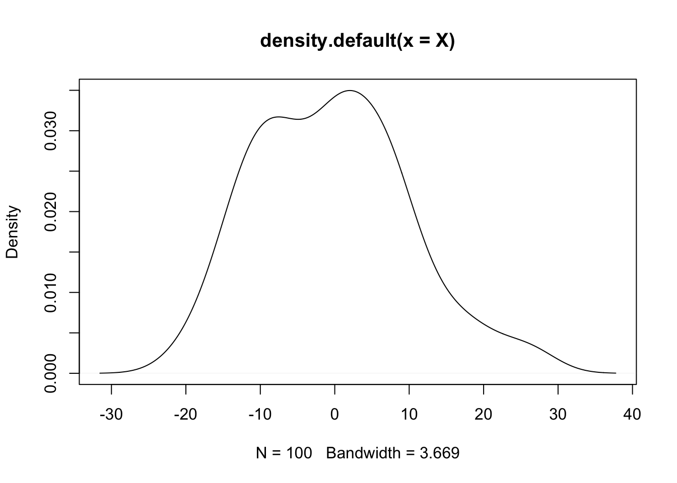
glm.nb()function is an updated version ofglm()function with a functionality of estimation of parameterthetafor a Negative Binomial generalized linear model.formula: an argument for the
glmfunction.link: a link function
Code
# import the data
ships <- MASS::ships %>%
    filter(service > 0)

# run glm.nb() function
ship.nb0 <- MASS::glm.nb(incidents ~ 1 + offset(log(service)), data = ships)
summary(ship.nb0)
##
## Call:
## MASS::glm.nb(formula = incidents ~ 1 + offset(log(service)),
## data = ships, init.theta = 2.923204332, link = log)
##
## Deviance Residuals:
## Min 1Q Median 3Q Max
## -1.9194 -0.9286 -0.5283 0.3488 2.4190
##
## Coefficients:
## Estimate Std. Error z value Pr(>|z|)
## (Intercept) -5.7181 0.1377 -41.53 <2e-16 ***
## ---
## Signif. codes: 0 '***' 0.001 '**' 0.01 '*' 0.05 '.' 0.1 ' ' 1
##
## (Dispersion parameter for Negative Binomial(2.9232) family taken to be 1)
##
## Null deviance: 35.809 on 33 degrees of freedom
## Residual deviance: 35.809 on 33 degrees of freedom
## AIC: 173.38
##
## Number of Fisher Scoring iterations: 1
##
##
## Theta: 2.92
## Std. Err.: 1.21
##
## 2 x log-likelihood: -169.378odTestfunction compares the log-likelihood of a negative binomial regression model and a Poisson regression model frompscllibrary. It has arguments as follows:glmobj: an object of
negbinalpha: significance level
digits: number of digits
Code
# odTest for the negative binomial
pscl::odTest(ship.nb0)
## Likelihood ratio test of H0: Poisson, as restricted NB model:
## n.b., the distribution of the test-statistic under H0 is non-standard
## e.g., see help(odTest) for details/references
##
## Critical value of test statistic at the alpha= 0.05 level: 2.7055
## Chi-Square Test Statistic = 74.817 p-value = < 2.2e-16zeroinflis a function fits zero-inflated regression models for count data through maximum likelihood frompscllibrary. It has arguments as follows:formula: symbolic description of the model
dist: a count model family; “poisson”, “negbin”, “geometric”
link: a link function in the binary zero-inflation model; “logit”, “probit”, “cloglog”, “cauchit”, “log”
Code
# data
articles <- read.csv("./Data/art.csv")
# run zero-inflated model
art.zip1 <- pscl::zeroinfl(art ~ fem + mar + kid5 + phd + ment | 1, data = articles, family = poisson)
summary(art.zip1)
##
## Call:
## pscl::zeroinfl(formula = art ~ fem + mar + kid5 + phd + ment | 1, data = articles, family = poisson)
##
## Pearson residuals:
## Min 1Q Median 3Q Max
## -1.5296 -0.9976 -0.3026 0.5398 7.2884
##
## Count model coefficients (poisson with log link):
## Estimate Std. Error z value Pr(>|z|)
## (Intercept) 0.685967 0.103522 6.626 3.44e-11 ***
## femWomen -0.231609 0.058670 -3.948 7.89e-05 ***
## marSingle -0.131972 0.066130 -1.996 0.046 *
## kid5 -0.170474 0.043296 -3.937 8.24e-05 ***
## phd 0.002526 0.028511 0.089 0.929
## ment 0.021543 0.002160 9.973 < 2e-16 ***
##
## Zero-inflation model coefficients (binomial with logit link):
## Estimate Std. Error z value Pr(>|z|)
## (Intercept) -1.6813 0.1558 -10.79 <2e-16 ***
## ---
## Signif. codes: 0 '***' 0.001 '**' 0.01 '*' 0.05 '.' 0.1 ' ' 1
##
## Number of iterations in BFGS optimization: 13
## Log-likelihood: -1621 on 7 Df4.5 Exercise & Quiz
4.5.1 Quiz: Exercise
- Use “Quiz-W4: Exercise” to submit your answers.
Add an interaction between married and female; interpret the interaction in terms of relative risk.(link to exercise 1)
Hand calculation: For a married female student with two children under 6, whose mentor has 8 publications and the phd program prestige score being 3, calculate the expected number of papers published during the last three years of PhD.(link to exercise 2)
Refit the above model without the exposure offset. Describe any problems you see. (link to exercise 3)
Is the function
glm.dispuseful for testing a binomial distribution for overdispersion. Could it be made to be so? How?. (link to exercise 4)Consider drawing Y = 10 from the negative binomial; hypothesize a \(\nu_i\) (from the plot of the Gamma draws) for this particular draw from the negative binomial (most recent) plot. (link to exercise 5)
4.5.2 Quiz: R Shiny
- Questions are from R shiny app “Lab 3: Count data”.
- Use “Quiz-W4: R Shiny” to submit your answers.
[The no-predictor model]
- Compute the exponentiated intercept Use the glm function with the argument family = poisson to do this.
[Adding predictors]
- Calculate the sample variance by gender and checked all that applies
[Interpreting Poisson coefficients]
Which variable does not predict article count well? (That is, which one is not statistically significant at \(\alpha\) =0.05 ?) Exponentiate the coefficient on this variable. How do you interpret this value?
What does the Poisson regression model with the quadratic term in the variable “ment” tell us?
[Overdispersion]
- Compute and print \(\phi\) for the quadratic Poisson model
[Negative binomoal regression]
- What does this tell you about the dispersion of the outcome? (see handouts for variance formula)
[Making predictions under ZIP regression]
- Compute the marginal probability of publishing zero articles and the actual fraction of zeroes observed in the data.
4.5.3 Quiz: Chapter
Use “Quiz-W4: Chapter” to submit your answers.
Compute the probability of observing 5 counts assuming Y follows a Poisson distribution with parameter lambda equals 3.5.
Compute the variance of the Poisson distribution from Q3
Select a FALSE statement
What is a benefit of using Quasi-Poission model?
In order to run the Poisson regression using ‘glm’ function in R, what ‘LINK’ function should you use?
Using the table result, what is the effect (relative risk ratio) associated with marriage status (marSingle==1)?
Calculate the expected number of papers published during the last three years of PhD for a married female student (fem==1 & marSingle==0) with 1 child under 6, whose mentor has 20 publications and the phd program prestige score being 2.
[Please select the right value for the blank] For every additional number of children, we expect _____ times the odds of being in the non-production group.
ZIP Poisson model has developed to deal with “excess zeros” issue, a form of over-dispersion. Compute the probability of “zero” in the model. You should use R (predict command) or Lab 3
[BONUS] What is the way in which the ZIP Poisson model computes the probability of “zero” in the model?
When all of the predictors are categorical this model forms a class of models known as log-linear models for count data. Agresti has written many books on the subject.↩︎
Note: Without multiple observations, we will not be able to estimate \(\nu_i\) for each individual, but we can estimate a variance across them.↩︎
Note:
Rparametrizes the negative binomial distribution a bit differently than STATA or SAS. With \(\theta\) in the denominator of the Gamma variance.↩︎Note: use of AIC/BIC depends on proper evaluation/implementation of the likelihood function as the normalizing constant matters in the non-nested case. We proceed assuming these packages allow for such comparisons, but acknowledge this potential limitation.↩︎