Chapter 3 Value of Data Analytics in Field Development Project (VOI Analysis)
3.1 Background
The concept of Value of Information (VOI) first was used in Oil&Gas industry in making decision related for drilling the reservoir(Grayson 1960). This concept originally comes from Decision Analysis (DA) community . (Schlaifer 1959) first defined the concept of Value of Information in the context of business decisions. More recently, (Bratvold et al. 2009) provided the overview the application and future recommendation of applying VOI analysis in the oil and gas industry. (Eidsvik, Mukerji, and Bhattacharjya 2015) has provided the overview of the use cases of the VOI in the earth science applications. According to the (Bratvold et al. 2009) any information gathering is concerned with two fundamental uncertainties,
- The uncertainties we hope to learn about it,but can not directly observe it
- The test result, which we refer to as the observable event
Genteelly, in this discussion (as well in the included codes), we denote the x to the distinction of the interest and y denote the observable distinctions.
The VOI is the defined as the "maximum value the decision maker should pay for additional information gathering regarding to the distinction of interest (x), and is defined as the below,(considering the risk neutral case):
VOI = EV with additional Information - EV without additional
Here, the EV means the Expected Value of the Decision. For example, for this particular context of decision making (Figure 3.1), assuming the three outcomes, the Value of Information can be shown mathematically as the Equation 6.2:
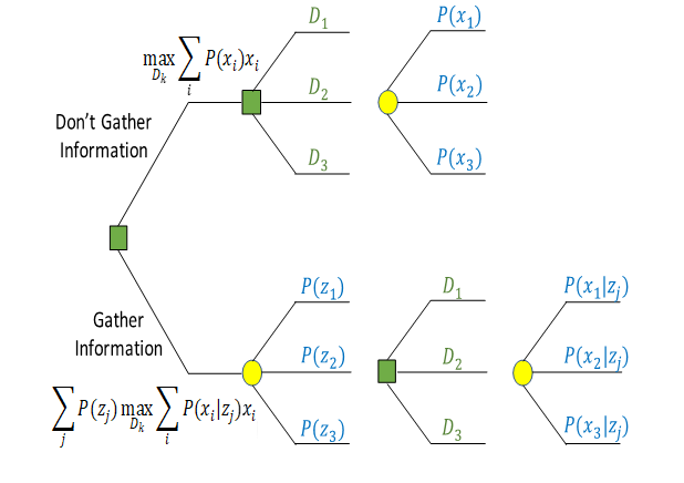
Figure 3.1: Decision Context for the Oil Company (without and with information)
\[\begin{equation} VOI = \sum_{j=1}^{N} P(z_{j}).max(\sum_{i=1}^{N} P(x_{i}|z_{j})x_{i},v) - max(\sum_{i=1}^{N} P(x_{i})x_{i},v) \tag{3.1} \end{equation}\]
Where,
- D_k: denotes alternative k for a decision,
- x_i denotes realization i of payoff,
- z_j denotes realization j of information signal (a test result),
- P(x_i) is the probability of payoff x_i before gathering information z_j (i.e., P(x_i) denotes the prior),
- P(x_i|z_j) is the conditional probability of payoff x_i given information signal z_j (i.e., P(x_i|z_j) denotes the posterior),
- and P(z_j) is the marginal probability of information signal z_j (i.e., P(z_i) denotes the preposterior).
VOI analysis, helps us in providing the framework to distinguish the constructive than wasteful information gathering process. Considering six dimension of the high-quality decision making (Figure 3.2), it could be considered that the ML developed in the previous chapter, work as information with updating our prior belief regarding decision to develop (start drilling) the field or walk away from the development.
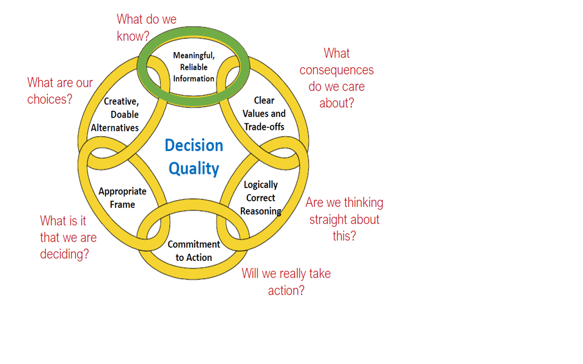
Figure 3.2: Six Dimesnions of High-Quality Decision Making
This decision considering the three possible outcomes Low, Medium, High (In the term of the it’s NPV value that again depends on well locations and injection scenarios) can be depicted in the Figure 3.3 . In this case the decision maker has two decision to make, whether to drill or walk away(It was considered the walking away the decisions no cost to the decision maker in this case.)
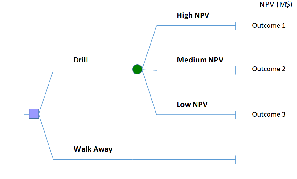
Figure 3.3: Simple Decision Tree for the Case of the Making Decision for Drilling 5-Spot Pattern (discussed in chap2)
3.2 High-Resolution Probability Tree Method (HRPT) for VOI Analysis
In this, we will use the High-Resolution Probability Method (HRPT) developed by (Bratvold, Thomas, and others 2014). First, to demonstrate this techniques, we use the HRPT method for one simple decision context with the known analytical solution and then we apply this method in the decision context described in the Figure 3.4. In this example, we suppose that a risk-neutral Oil company is considering drilling a well in an undeveloped area where the outcome (Net Present value) in this case is normally distributed with the mean of the \(\mu = 10MM\) and \(SD=20MM\), in Dollar.
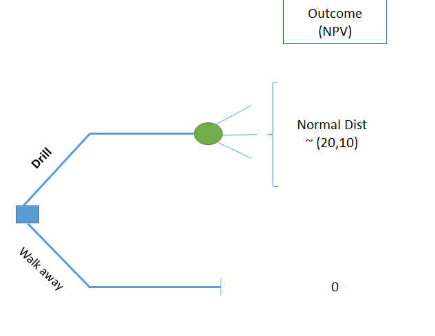
Figure 3.4: Decision Tree for TALL-N Problem (without information)
In the effort to make a better decision, the company considering the acquisition of seismic survey. The expert in the company believes that the seismic results are correlated with true value of the well with the correlation coefficient of \(\rho = 0.6\). It is assumed that in this case, the signal (seismic survey) will have a normal distribution with the same mean and standard deviation ,Figure (3.5. Here the decision makers face three decisions to make,1) Start the Drilling 2) Walk away from the Drilling, 3) Gather the information about the uncertainty of the out put. However, the information gathering has a specific value to could add to the decision, (VOI) that need be analyzed before “Gathering the Information.”
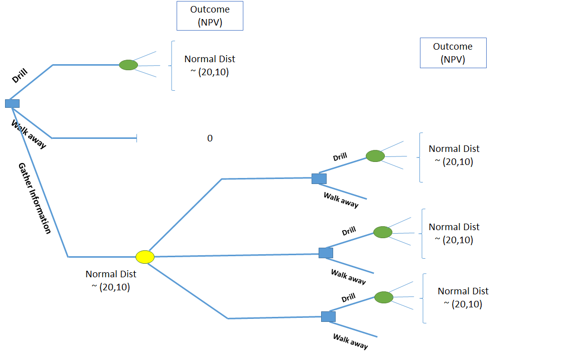
Figure 3.5: Decision Tree for TALLN Problem (with information)
Now, considering the prior distribution and signal distribution of this problem (is named TALL-N), Figure (3.6) shows both the prior distribution as well signal.
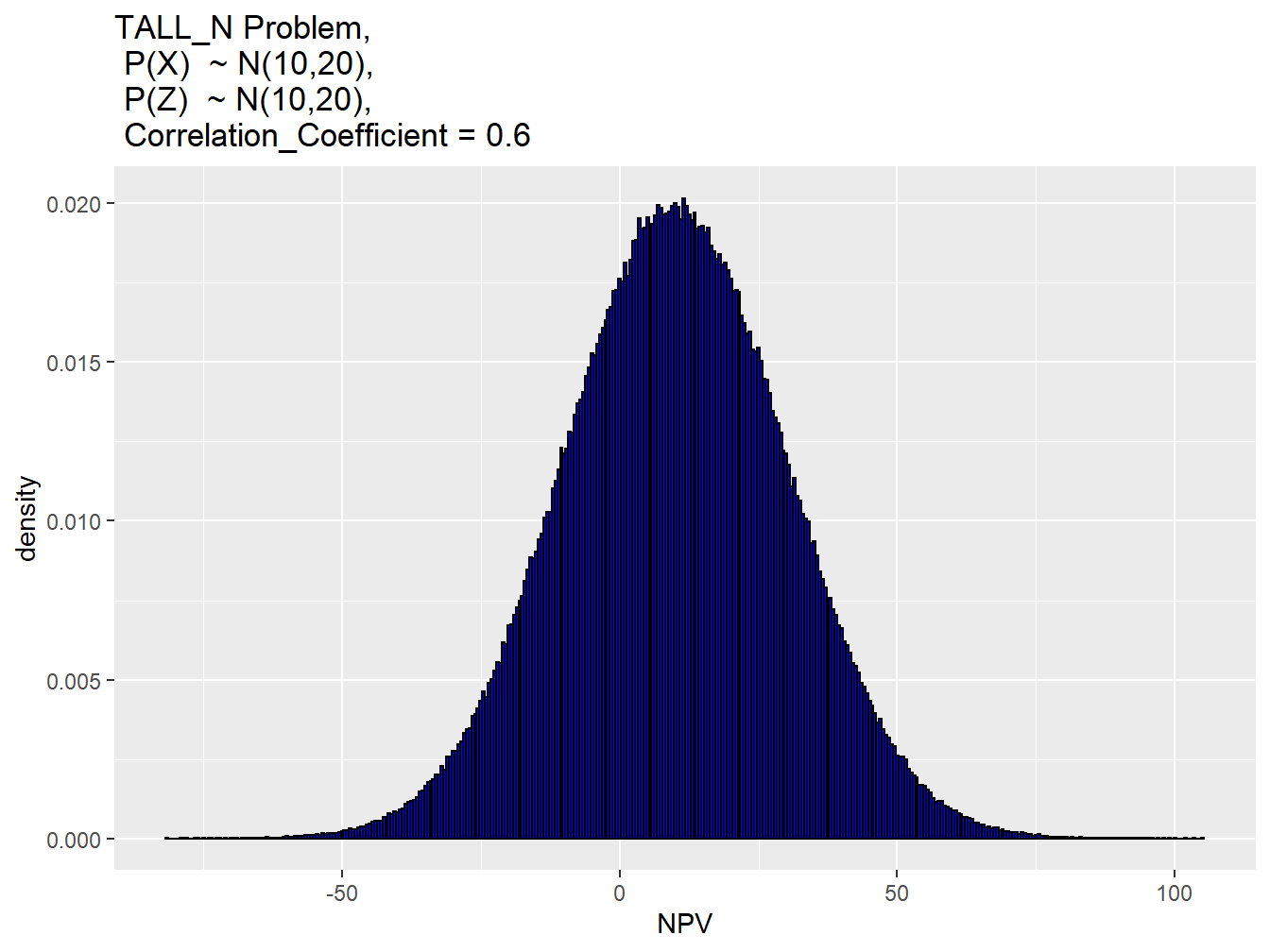
Figure 3.6: Permeability Distribution of the Field
Considering this information, Now we can use the (HRPT) method to calculate the Value of information (VOI) in this case. It is worth to mention that in this case, we used the the racket and mean method for discritizing the prior as well the signal distribution. In addition, the number of nodes (Nodes) in this case was 1000. Therefore, the the conditional probability will have the dimension of the 1000 in 10000.
Full other related data regarding this VOI case has been depicted in the Table 3.1.
| Parameter | Value |
|---|---|
| Mean Prior(x_mean) | 10.0 |
| Standard Deviation (Prior) | 20.0 |
| Mean Signal (z_mean) | 10.0 |
| Standard Deviation Signal (z_sd) | 20.0 |
| Correlation Coefficient (rho) | 0.6 |
| Cost | 0.0 |
| VOI | |
|---|---|
| Value of Information (VOI) is: | 1.35953174492042 |
On the other hand we know that this TALL_N problem has a analytical solution as the follow:(Sethian 1996)
\[\begin{equation} \ EVII = \begin{cases} \rho\sigma[\phi(\rho^{-1})c -\rho^{-1}c\psi(-\rho^{-1}c)] & \quad \text{if } , {\mu>v} \\ \rho\sigma[\phi(\rho^{-1})c +\rho^{-1}c\psi(\rho^{-1}c)] & \quad \text{if } , {\mu<v} \end{cases} \tag{3.2} \end{equation}\]
Where the, \(\mu\) is the mean of the prior; \(\sigma\) is the standard deviation of the prior; \(v\) is the value of alternative decision-the best decision without gathering more information); \(c=(\mu-v)/\sigma\) is known as the “coefficient of the divergence”; \(\sigma\) is the standard normal probability density function ; \(\psi\) is the standard normal cumulative distribution function, \(\rho\) is the positive correlation coefficient between the prior and the observed signal obtained through information system.
Here, the result of HRPT method and as well exact solution were found and the comparison of these two results has been made in the Figure @ref(fig:compa. The comparison was made to capture also range of the correlation coefficient and gain the number of nodes in discritization method in this case was (nodes=1000). In context of the TAll_N problem, the Table provide the value of the VOI found from the HRDT method, Exact solution and the (@ Bratvold, Thomas, and others 2014) paper.
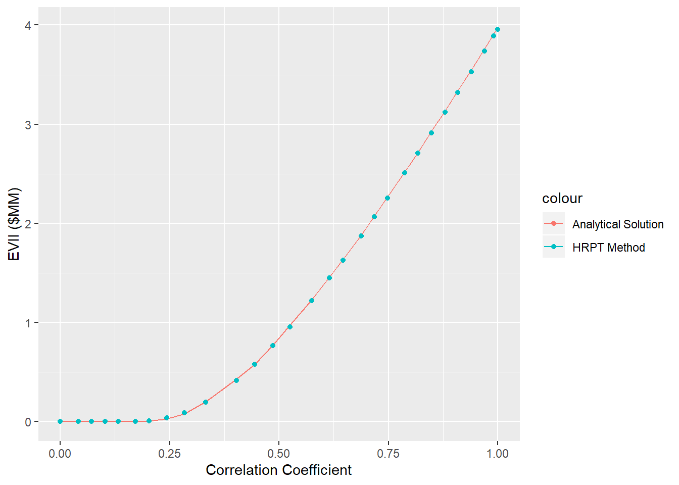
Figure 3.7: Comparison of the VOI found in Analytical Solution Vs. HRPT Method
3.3 Sensitivity Analysis of VOI to Prior, Likelihood and CAPEX
In VOI discussion, the value of information must be assesd before gathering the information. This provides insight to the decision maker about the maximum value that worth to pay for gathering the data. Here, in the context of the Machine Learning the cost of Information includes the following:
- Data Acquisition
- Pattern Detection
- Pattern Recognition
- Pattern Exploration
- Pattern Exploitation
On the other hand, the reliability of the ML model can be evaluated only if after acquisition of data and building the ML model. However, in the concept of VOI, the value of information must be asses before gathering the data. Therefore, we make a sensitivity analysis not only on the reliability of the result of data analytics (ML model) but also to the prior and as well CAPEX of the project. It must be mention that in the VOI analysis, the outcome of the event NPV is defined as the follows that includes the CAPEX cost (All the spending cost of the development project before production of the field):
\[\begin{equation} NPV=\sum_{k=1}^{n_T} \frac{[q_o^{k}P_o - q_w^k P_w -I^k P_{wi} ]\bigtriangleup t_k}{(1+b)^{t_k/D}} -CAPEX \tag{3.3} \end{equation}\]
Now, the discussion above aims to provide the framework to find the VOI in the cases of different scenarios for the following parameters:
- Mean of Prior Distribution
- Standard Deviation of Prior Distribution
- CAPEX (Capital Cost)
- Reliability of the Information
Mean of Prior Distribution:
In the work developed in the Chapter 2, we had 5000 total training set. These data-set represents the historical data set for this specific ‘5-Spot Pattern’. Well, in fact the prior is defined as the *historic data’ and ‘Expert Knowledge’, in this work while we consider the ‘Historic data’ as the prior, we will have different cases to include the several scenarios of the Prior distribution. To get the hint regarding which range of the prior distribution to be considered in sensitivity analysis, first we have look on the historical data-set of the 5-spot patter. The Figure 3.8 shows the histogram of the NPV of ‘Historical’ data-set. The box plot of this distribution was plotted in Figure 3.9. we can see that the historical data has the shape of the Normal distribution with the mean of 54 MM$ and standard Deviation of the 5.6 MM.
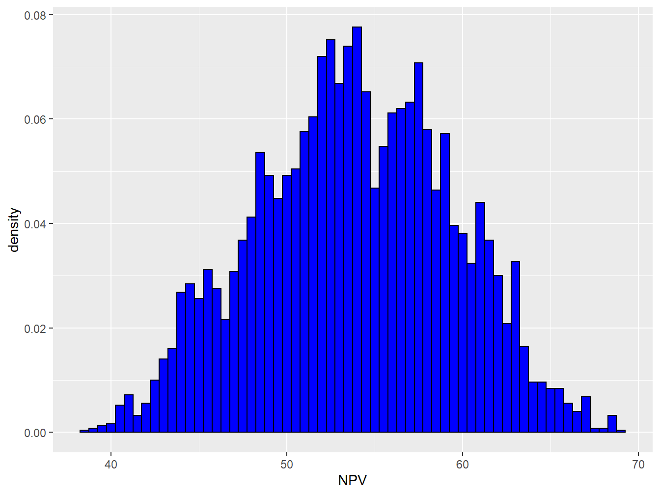
Figure 3.8: Distribution of the Historical NPV
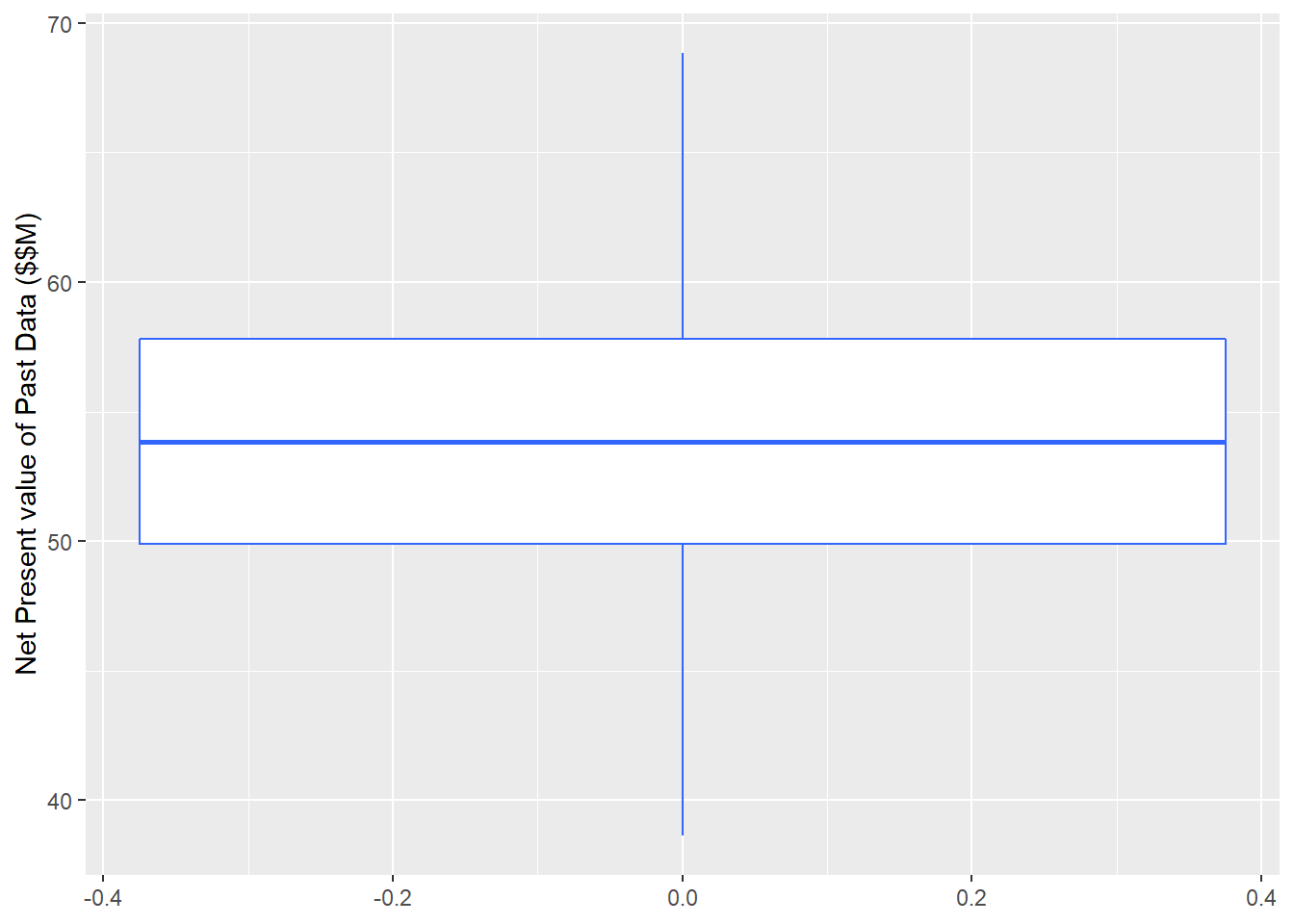
Figure 3.9: Box Plot of Permeability Distribution
Now this gives us the idea about the different scenario of the prior we could have in the sensitivity analysis. In this work, we considered 5 different possible cases for prior distribution. As shown in the Figure 3.10, these five distribution were considered as the possible scenarios of the prior (all in $MM):
- Normal Distribution, \(\mu = 30\)
- Normal Distribution, \(\mu = 40\)
- Normal Distribution, \(\mu = 50\)
- Normal Distribution, \(\mu = 60\)
- Normal Distribution, \(\mu = 70\)
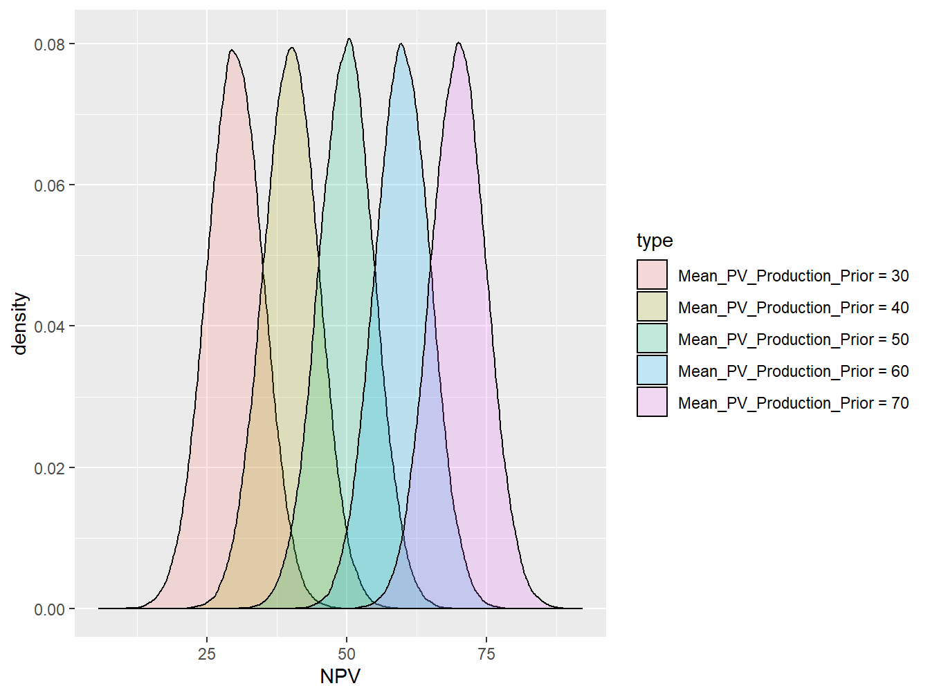
Figure 3.10: Range of Prior Distribution in VOI Analysis-Normal Distribution
Standard deviation of Prior Distribution:
However, considering the only different mean values of the prior distribution is not sufficient. Therefore, in this study we considered the both the change in the mean and as well spread of the data from the mean with considering the 4 different possible standard deviation. Again, as it was discussed in the for the mean analysis, we had the look on the standard deviation of the “Historical data” to get the insight about the range of the standard deviations to be included in the sensitivity analysis. The Standard Deviation of the the past data-set was, \(SD=5.6\), then the following were considered for the range of SD values. (Note: Each mean prior, will have 4 different SD values in the analysis, therefore, the total number of the prior distribution are \(5*4=20\) ).
- Normal Distribution, \(sd = 2.5\)
- Normal Distribution, \(sd = 5\)
- Normal Distribution, \(sd = 10\)
- Normal Distribution, \(sd = 15\)
The Figure 3.11 shows the 4 different assigned standard deviation at the mean prior distribution of the \(\mu = 50\).
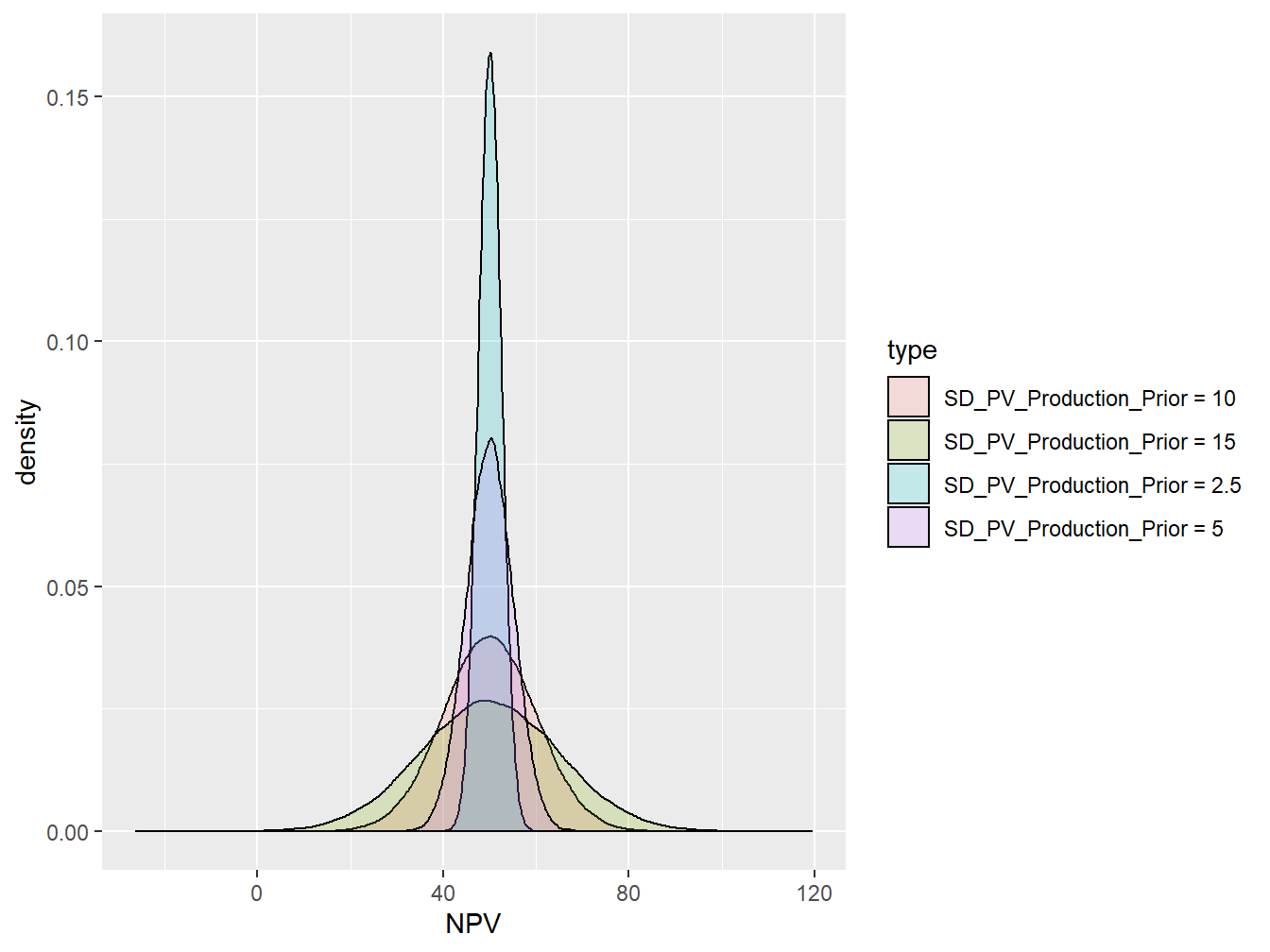
Figure 3.11: Prior Distribution for Four SD Values at Mean = 50 MM(Dollar)
CAPEX:
The evaluation of the CAPEX (Capital Cost before the oil production) must be done through economic expert of the the decisions. Since the NPV defined in this case is all consider the money discount factor, the CAPEX values in this study as well must be expresses in the Net Present Values, that is why we call the CAPEX in the figures as PV_CAPEX Here, We considered the four possible range for the CAPEX in order to capture the range of CAPEX values, these are as follows (in MM$):
- CAPEX \(PV(Capex) = 30\)
- CAPEX, \(PV(Capex) = 40\)
- CAPEX, \(PV(Capex) = 50\)
- CAPEX, \(PV(Capex) = 60\)
The Figures (3.12, 3.13,3.14,3.15) show the results of sensitivity analysis of the VOI at different standard deviation of the prior, SD=2.5,5,10,15. For example when we have a normal distribution withe the SD = 2.5, the decsion context with the following characteristics,:
- Mean of prior distribution: 50 MM (Dollar)
- Correlation Coefficient: 0.8
- CAPEX: 50 MM (Dollar);
The VOI for this case is equal to 0.8 MM (Dollar). In addition we can see two different trends:
- The VOI increases with increasing the reliability of the information (Correlation Coefficient)
- The VOI has the highest value when the CAPEX is equal to the mean of the prior distribution, showing that the VOI is more valuable when it has stronger capability to change our decisions.
- With increasing standard deviation values, the VOI get more valuable. The main reason that could be attributed is that in the case of high standard deviation, there is more down side in distribution of the prior, so that the reliable information could be more valuable in order to avoid that downside.
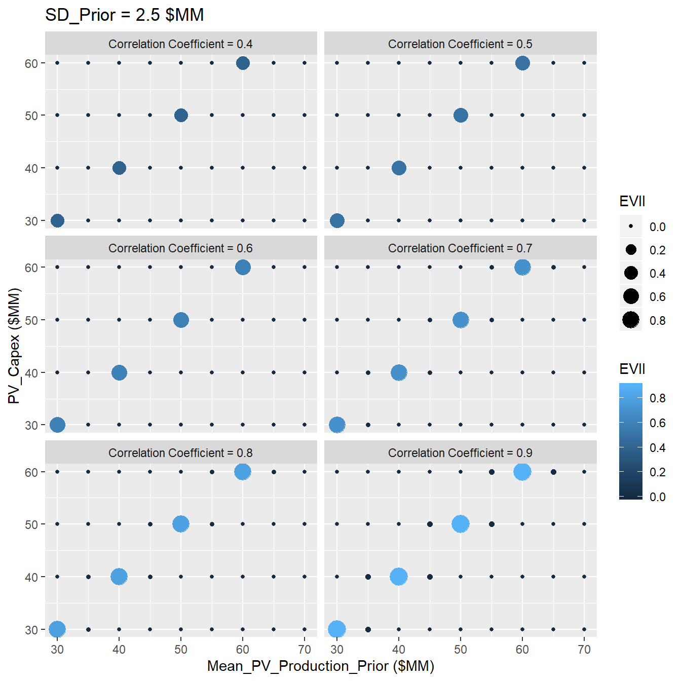
Figure 3.12: Sensitivity Analysis of VOI at SD=2.5
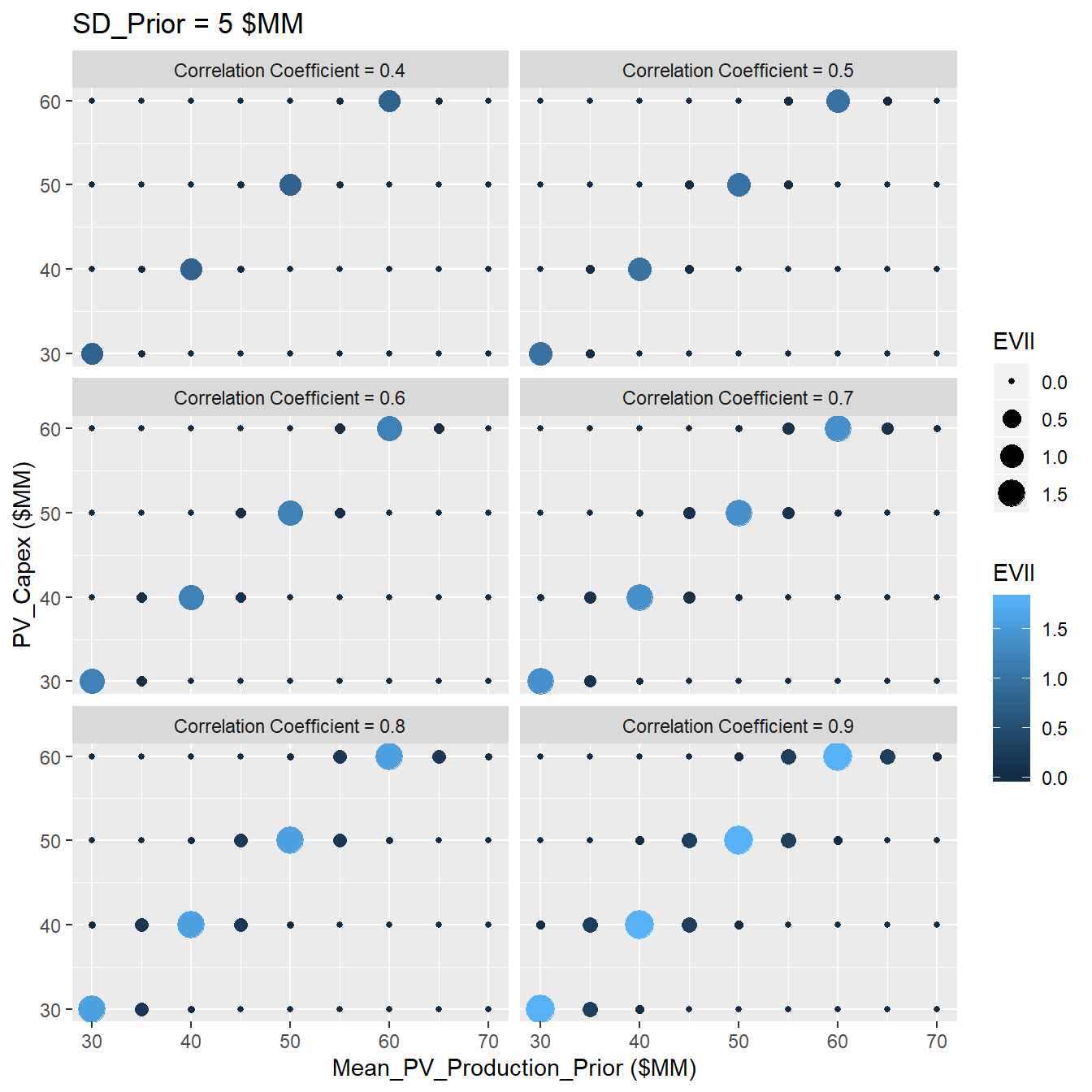
Figure 3.13: Sensitivity Analysis of VOI at SD=5
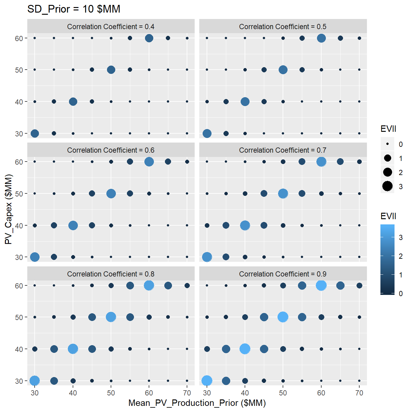
Figure 3.14: Sensitivity Analysis of VOI at SD=10
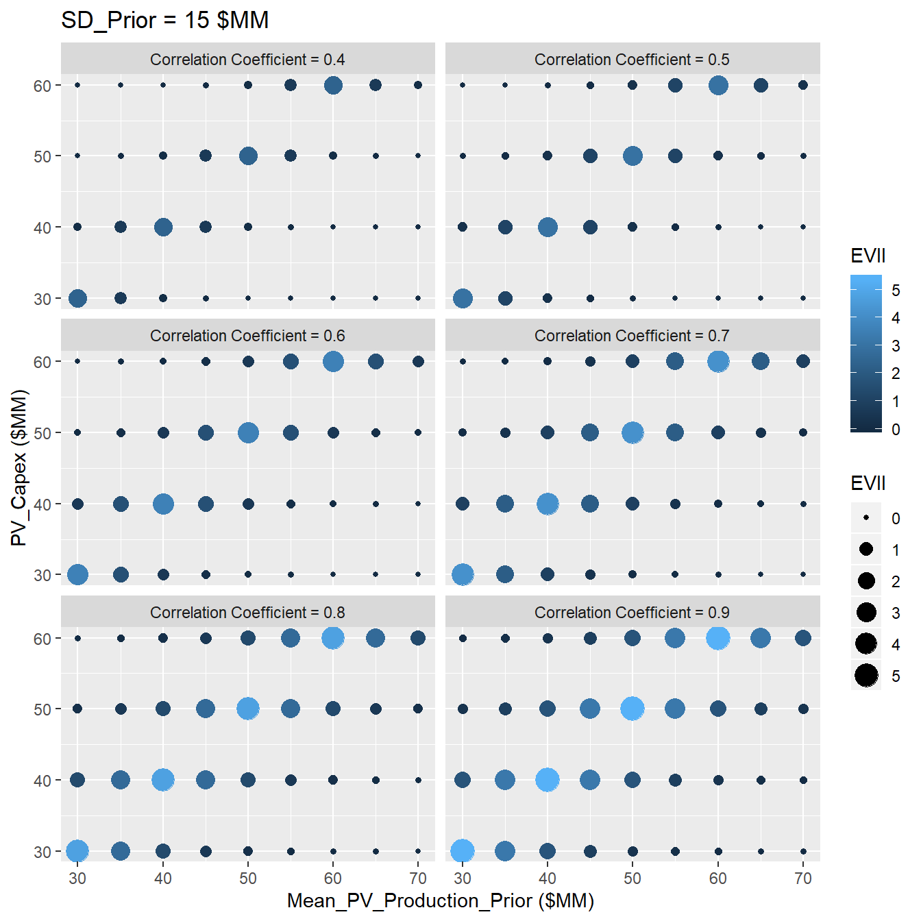
Figure 3.15: Sensitivity Analysis of VOI at SD=15
References
Bratvold, Reidar B, J Eric Bickel, Hans Petter Lohne, and others. 2009. “Value of Information in the Oil and Gas Industry: Past, Present, and Future.” SPE Reservoir Evaluation & Engineering 12 (04). Society of Petroleum Engineers: 630–38.
Bratvold, Reidar Brumer, Philip Thomas, and others. 2014. “Robust Discretization of Continuouos Probability Distributions for Value-of-Information Analysis.” In International Petroleum Technology Conference. International Petroleum Technology Conference.
Eidsvik, Jo, Tapan Mukerji, and Debarun Bhattacharjya. 2015. Value of Information in the Earth Sciences: Integrating Spatial Modeling and Decision Analysis. Cambridge University Press.
Grayson, Charles Jackson. 1960. Decisions Under Uncertainty: Drilling Decisions by Oil and Gas Operators. Ayer.
Schlaifer, Robert. 1959. “Probability and Statistics for Business Decisions.” McGraw-Hill.
Sethian, James A. 1996. “A Fast Marching Level Set Method for Monotonically Advancing Fronts.” Proceedings of the National Academy of Sciences 93 (4). National Acad Sciences: 1591–5.