Chapter 4 Robust Field Development Optimization Using the Proxy Model
4.1 Introduction
So far, in the chapter 2 we developed a proxy model utilizing machine learning algorithm. In the chapter 3, we discussed the Value of Information in decision making for field development project. In this chapter the optimization algorithm will be utilized to optimize the field development scenario. This chapter presents a robust ,multidimensional, simultaneous optimization of well locations and controls (injection rate) using a Genetic Algorithm (GA) type of Evolutionary Algorithm (EA). Here, we demonstrate the robust optimization (RO) to the 5-spot pattern. This optimization algorithm is developed to fully take advantage of the computational efficiency and speed of the proxy model. Within a Robust Optimization procedure, the geological uncertainties are included by set of realizations generated using the geostatistical methods. Then, the objective of RO is to find a control vector (here both injection wells coordinates and water injection scheme) that optimize the expected value (EV) of the objective function (NPV) over the all geological realizations. This workflow of is named RO since optimum control vector is robust to geological uncertainty. (Hong, Bratvold, and Nævdal 2017,@van2009robust)
4.2 Brief Summary of the Proxy-Model
We begin with a summary of the approach presented in Chapter 3. As with other machine learning algorithm, the procedure starts with the collection and manipulation of feature and response data. This is achieved by running reservoir simulations using randomly sampled well locations within the domain of interest. It must be noted that special care has been taken to not to avoid inefficient well placement of injectors leading to weak sweep efficiency. The injectors are not only have distance from the producers as well as are in distant place from each other.
For each training observation, well-to-well connectivities and Pore Volume (PV) of flight are computed between every pair of wells in the reservoir using FMM. Together, these parameters make up the predictor variables that constitute the feature labels used for training. Each each training, characterized by a unique well configuration and combination of predictor parameters, is evaluated in a reservoir simulator to obtain a true output. A well known reservoir-wide objective function, net present value (NPV), can then be computed from the simulator output, to comprise the corresponding response observation. Then, the feature and response data are fed into the XGBoost algorithm to create a prediction model. Tuning parameters for the XGBoost algorithm (number of trees, shrinkage factor, bag fraction, and tree depth) are optimized by cross-validation to minimize the mean square error and avoid over-fitting.
4.3 Robust Optimization of Well Placement and Water Injection Scheme
The manner in which the joint problem has been handled in recent studies has varied. (Essen et al. 2009) considered the geological uncertainty in optimization water-flooding using a gradient-based optimization which the gradients are obtained with an adjoint formulation.(Chen et al. 2009) proposed a ensemble-based optimization method(EnOpt) which is adjoint-free and gradient is approximated by the co-variance between the control variables and objective function. (Forouzanfar and Reynolds 2014) conducted a joint optimization in which both the location and injection schemes are handled using gradient projection. (Bellout et al. 2012) proposed a hybrid approach where well placement was solved using derivative-free methods based on pattern search while injection rate is solved by adjoint-based method. (Hong, Bratvold, and Nævdal 2017) proposed a Ensemble-based optimization (EnOpt) where the capacitance-resistance model (CRM) was used as a proxy for optimization of injection scheme. (A. Nwachukwu, Jeong, Sun, et al. 2018) proposed a scheme similar Mesh Adaptive Direct Search (MADS)for joint optimization where Extreme Gradient Boosting method (XGBoost) was build for making forecast for given any set of observations.
In this chapter, we propose a Genetic Algorithm (GA) (Holland 1975,@goldberg1989genetic) as a stochastic search algorithm which are are able to solve optimization of problems of the and development of an optimization strategy that efficiently combines the proxy and a reservoir simulator to solve the joint well locations and controls problem in a multidimensional manner.following type:
\[\begin{equation} \Theta^{*} \equiv arg max f(\theta) = {\theta^{*} \in \Theta : f(\theta^{*})>f(\theta), \vee\theta \in \Theta } \tag{4.1} \end{equation}\]
Where \(\Theta\) \(\subseteq\) \(R\) defines the search spaces, \(\theta = (\theta{1},\theta{2},..,\theta{p})\) is domain of parameters where each \(\theta{i}\) varies between lower and upper bound. The joint Optimization in this work can be classified as the type of equation above where the \(S\) is the search space for (NPV) while the domain of parameters of the problem are defined as well locations and water injection scheme.(Scrucca and others 2013)
GA utilize evolutionary strategies inspired by the basic principles of biological adaption. At each stage of the evolution, a population is composed of a number of individuals, also called chromosomes or strings . each chromosomes is made of units (genes, features, characters) which control the inheritance of one or several characters. Genes of specific characters are placed along the chromosome, and the corresponding string positions are called loci. Each genotype would represent a potential solution to a problem. The decision variables, or phenotypes, in a GA are obtained by applying some mapping from the chromosome representation into the decision variable space, which represent potential solutions to an optimization problem. A suitable decoding function may be required for mapping chromosomes onto phenotypes.
The genetic algorithm process could be summarized as follow:
- type of variables, fitness function, GA parameters and convergence criteria must be defined to initiate the GA process,
- Initial random population of size n is generated, so for step k = 0 we may write \({\theta_{1}^{0},\theta_{2}^{0},...,\theta_{n}^{0}}\) .
- convergence criteria are checked and if it is meet, GA stops.
- The fitness of each member of the population at any step k, \(f(\theta_{i}^{k})\) is computed and probabilities \(p_{i}^{k}\) are assigned to each individual in the population, proportional to their fitness.
- The reproducing population is formed (selection) by drawing with replacement a sample where each individual has probability of surviving equal to \(p_{i}^{k}\).
- A new population\({\theta_{1}^{k+1},\theta_{2}^{k+2},...,\theta_{n}^{k+1}}\) is formed from the reproducing population using crossover and mutation operators.
- Then, set \(k = k + 1\) and the algorithm returns to the fitness evaluation step. When convergence criteria are met the evolution stops, and the algorithm deliver \(\theta^{*} \equiv argmax f(\theta_{i}^{k})\) arg max as the optimum. The flow chart of this algorithm is shown in the Figure 4.1.
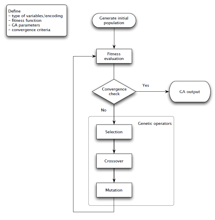
Figure 4.1: Flow Chart for Genetic Algorithem Process
4.4 Optimization Process
The proposed methods presented in the preceding sections were applied to a synthetic field under five spot pattern with 4 production wells and 1 injection well. Geological model were built on a 45 × 45 two-dimensional grid measuring 450 m on each side and 10 m in thickness. In order to take the geologic uncertainty into consideration, geological realizations were generated using Sequential Gaussian Simulation (SGS) (Pyrcz and Deutsch 2014) with the semivariogram parameters given in Table 4.1.
| Parameter | Value |
|---|---|
| Nugget Effect | Sill/2, md^2 |
| Type | Spherical |
| Range | 20 (grid cell) |
| Anistropy ratio | 1 |
| Azimuth | 0-degree (North) |
The geological model has the petrophysical uncertainty (in this case permeability) and 50 realizations were considered to capture the uncertainty. 10 realization (out of 50) of permeability of the reservoir has been shown in the Figure 4.2.
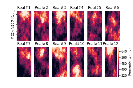
Figure 4.2: Twelve Realizations (out of 50) of Permeability in the Geological Model
Considering the Robust Optimization defined in the previous sections, the problem can be stated as the follows: The Optimization algorithem search solution(s) for injection well coordinates and water injection scheme to maximize EV(NPV) ove all realizations.
The GA optimization was conducted using the parallel Computing in R programming language with GA package. (Scrucca and others 2013) The initial setup of the algorithm (Optimization parameters) has been shown in the Table 4.2.
| GA Parameters | Value |
|---|---|
| Population Size | 25.0 |
| robability of crossover between pairs of chromosomes | 0.8 |
| Probability of mutation in a parent chromosome | 0.1 |
| Maximum Iteration | 20.0 |
| Number of consecutive generations without any improvement | 5.0 |
As reminder, the NPV value is calculated as the following:
\[\begin{equation} NPV=\sum_{k=1}^{n_T} \frac{[q_o^{k}P_o - q_w^k P_w -I^k P_{wi} ]\bigtriangleup t_k}{(1+b)^{t_k/D}} \tag{4.2} \end{equation}\]
In each iteration of GA algorithm, the fitness function is the mean NPV of all 50 realizations, defined as the below:
\[\begin{equation} EV(NPV(u)) = \sum_{i=1}^{n_r=50} \frac{NPV_{i}(u)}{N} \tag{4.3} \end{equation}\]
Where \(u\) in this case is the injection well coordinates and injection rate scenarios(defined in Chapter 3).
The EV(NPV(u)) is found using ML proxy developed in the Chapter2, in each iteration. The flow chart of the optimization process in this chapter can be depicted as the Figure 4.3.
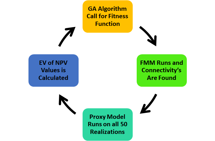
Figure 4.3: Flow Chart of the Optimization Alghorithem
4.5 Results of Optimization
After running the 500 (25*20) iterations ( which it means 25,000 proxy model iteration because of the 50 realizations), the result of the improvement in the best solution over the 20 generations could be found in the figure (4.4)
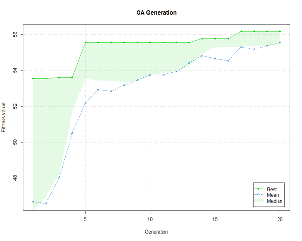
Figure 4.4: Evolution of GA Algorithem Solution over Generations
The best solution after 20 Iteration was found 56.7 $MM. This value is the mean NPV of the all realization at the U( Control vector) with the following parameters of the optimization in the Table 4.3.(Scrucca and others 2013)
| Componenet of u Vector | Value |
|---|---|
| X and Y Coordinate of Injector Number 1 | 3,19 |
| X and Y Coordinate of Injector Number 2 | 40,9 |
| X and Y Coordinate of Injector Number 3 | 9,41 |
| X and Y Coordinate of Injector Number 4 | 34,41 |
| Starting Rate of Injector Number 1 | 250 |
| Starting Rate of Injector Number 2 | 250 |
| Starting Rate of Injector Number 3 | 100 |
| Starting Rate of Injector Number 4 | 200 |
| Gamma Rate of Injector Number 1 | 0.001 |
| Gamma Rate of Injector Number 2 | 0 |
| Gamma Rate of Injector Number 3 | -0.005 |
| Gamma Rate of Injectior Number 4 | 0.005 |
Now, the other area that was studied in this work is at the optimum control vector, how much the the distribution of NPV found from the Proxy Model differs from the the results of the Numerical Reservoir Simulator at that optimum location. This result will provide some insight about what is the deviation of the result of optimum location in the proxy model compared to complex, physics based model. The Figure 4.5 shows the distribution of the NPV over 50 realizations. The blue and red vertical lines are representative of the mean values.
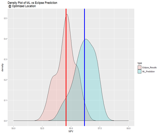
Figure 4.5: Comparison of the NPV Found (at Optimum Locations) in Machine Learning Vs. Numerical Simulator
Finally, we analyze the Value of Complexity in this case. The Value of Complexity is defined as:
- Value Of Complexity = Value Created from Rich Model - Value Created from Physics-Reduced Model*
This Difference, that in this study is shown with the difference in the NPV values of the Machine Learning Model and Eclipse reservoir Simulator has shown in the Figure 4.6
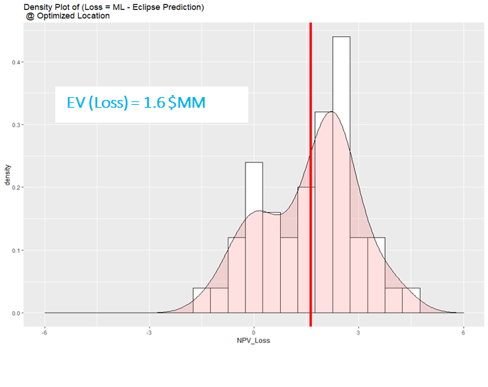
Figure 4.6: Value of Complexity (Deviation of Proxy Model from Complex One)
References
Bellout, Mathias C, David Echeverría Ciaurri, Louis J Durlofsky, Bjarne Foss, and Jon Kleppe. 2012. “Joint Optimization of Oil Well Placement and Controls.” Computational Geosciences 16 (4). Springer: 1061–79.
Chen, Yan, Dean S Oliver, Dongxiao Zhang, and others. 2009. “Efficient Ensemble-Based Closed-Loop Production Optimization.” SPE Journal 14 (04). Society of Petroleum Engineers: 634–45.
Essen, Gijs van, Maarten Zandvliet, Paul Van den Hof, Okko Bosgra, Jan-Dirk Jansen, and others. 2009. “Robust Waterflooding Optimization of Multiple Geological Scenarios.” Spe Journal 14 (01). Society of Petroleum Engineers: 202–10.
Forouzanfar, Fahim, and AC Reynolds. 2014. “Joint Optimization of Number of Wells, Well Locations and Controls Using a Gradient-Based Algorithm.” Chemical Engineering Research and Design 92 (7). Elsevier: 1315–28.
Holland, John H. 1975. “Adaptation in Natural and Artificial Systems Ann Arbor.” The University of Michigan Press 1: 975.
Hong, AJ, RB Bratvold, and G Nævdal. 2017. “Robust Production Optimization with Capacitance-Resistance Model as Precursor.” Computational Geosciences 21 (5-6). Springer: 1423–42.
Nwachukwu, Azor, Hoonyoung Jeong, Alexander Sun, Michael Pyrcz, Larry W Lake, and others. 2018. “Machine Learning-Based Optimization of Well Locations and Wag Parameters Under Geologic Uncertainty.” In SPE Improved Oil Recovery Conference. Society of Petroleum Engineers.
Pyrcz, Michael J, and Clayton V Deutsch. 2014. Geostatistical Reservoir Modeling. Oxford university press.
Scrucca, Luca, and others. 2013. “GA: A Package for Genetic Algorithms in R.” Journal of Statistical Software 53 (4). Citeseer: 1–37.