Chapter 2 Development of Proxy Model (Less Rich Model) Using a Machine Learning
2.1 Introduction
Proxy reservoir models [^1] traditionally have been used as a computationally efficient method to simulate reservoir and well responses in subsurface modeling. The advantage of this area of application is that parts of the governing physics can be modified to a simpler mathematical equations, or through the use of data-driven methods, thereby sacrificing some accuracy for a significant decrease in the computational time and resource needed. This fast, computationally inexpensive model is especially very useful during the optimization process where iteration in the order of several thousand is required. Herein, we classify the proxy models in the two main categories, physics-based and data-driven approaches.
2.1.1 Physics-Based Proxies
Physics-based proxies incorporate the mathematics of fluid flow in a simpler framework using assumptions that may be deemed appropriate for the situation. Examples of this approach include capacitance-resistance (CRM) modeling which is based on material balance and derived from total fluid connectivity. (Sayarpour et al. 2009), the Fast Marching Method (FMM)(Sethian 1996, @sharifi2014dynamic) and random walker particle tracking (RWPT)(Stalgorova, Babadagli, and others 2012). (Sayarpour et al. 2009) used CRM to characterize the resevoir response based on inter-well connectivity. These connectivities, as will be discussed in the rest of this chapter, present a an efficient way to densely include the reservoir geology without explicitly invoking the petrophysical properties of the field. However, as opposed to static connectivities that are used in this work (In CRM model, history matching is performed to calculate connectivities; while in FMM connectivities are found using before production.). In CRM model connectivity are dependent not only on the static reservoir geology, but on the dynamic injection and production rates.
2.1.1.1 Data-Driven Based Proxies
Over the last decades, data-driven based proxies have increased dramatically in popularity, owing to recent advances in big data and a broad wave of emerging ‘Machine Learning’ applications in research and industry. This class of proxies have a entirely data-driven approach, in which a sets of of data observations are trained for forecasting of reservoir out without relying on any specific physical equatipons. The training data set used for training the model could be found from field measurements, or synthesized using a commercial reservoir simulator. Most studies in this area have used artificial neural networks (ANN) (Ahmadi et al. (2013)),(Yu, Zhu, and Diao 2008), as the learning algorithm, although implementation of tree-based methods such as random forests and gradient boosting is common. (Castelletti et al. 2010)
2.1.2 Data-Driven or Physical Based-Proxy?
Whether using the physics-based proxy or data-driven proxy, one should keep in mind the statement of the George Box(Box 1979), “All models are wrong, some are useful.” Therefore, the main purpose of the models are to support the decision maker with providing the insight. On the other hand, (Bratvold et al. 2009),noted that “O& G companies tend to build too much detail in their decision-making models from the beginning”. Here, considering the voluminous codes and models in the commercial simulators, the work tends to build proxy model (less rich model) to help decision makers make a decision in a ‘timely’ manner. Then, choosing between “Data-Driven” or “Physic Based” proxy, herein the research take fully advantages of the both methods in the new method named “Hybrid Proxy”. In this work the proxy is neither fully data-driven nor physical based, but combination of the both. In fact, in the hybrid approach, we calculate the ‘Features’ of the ML algorithm using the physical-based approach while then we take advantage of the recent advance in pattern recognition techniques (Machine Learning), to find the pattern between those ‘Features’ and response of the reservoir. The Fast Marching Method (FMM) introduced by (Sethian 1996) and has been used to compute travel times of the pressure front from a source/sink (Sharifi et al. 2014) often called ‘diffusive times of flight’ are the features used in this work driven from physic-based analytical method.(A. Nwachukwu, Jeong, Pyrcz, et al. 2018)
2.2 Workflow
In this chapter the method used to build the proxy model will be explained. The methodology to build this proxy model can be explained in the six steps. First, we provide the brief summary of this methodology but in the next pages more complete description of the each step will be further explained. The flow diagram of the development process has been depicted in the Figure 2.1. The development of this proxy consist of the following steps:
Geological model and the type of field development scenario (five spot pattern or any injection scenario) should be specified.
After specifying the model, the Sequential Gaussian Simulation (SGS) is performed to build the different realizations the petrophysical parameter. (In this work, the permeability was defined as the source of uncertainty and different realizations are representative of the uncertainty in the permeability data)
In each realization, the Fast Marching Method (FMM) is performed to find the connectivities between injectors and producers, between injectors and pore volume of the flight.
The realizations in step 2 with it’s injection scenario are fed to the numerical simulator to produce the monthly Oil production, water injection and water production as the result forward fully physic-based model.
In this step, the output of numerical simulator is post processed to extract the monthly production of water and oil.
At last step, we calculate the Net Present Value (NPV) of the development scenario to be used as the output of the ML algorithm.
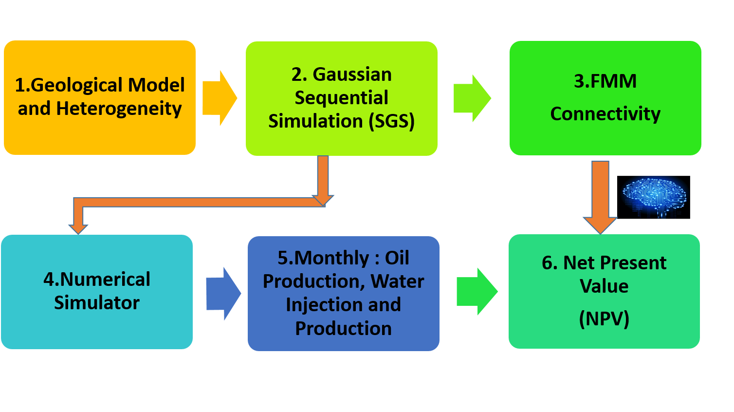
Figure 2.1: Flow Diagram of Development of the Proxy Model
2.2.1 Geological Model and Heterogeneity
In this work, two-dimensional reservoir geometry with two phases water/oil system was considered. The grid based geological model with size of the \(45*45\) was used in this work. The parameters of the model and rock and water properties have shown in the Table 2.1.
| Parameter | Value |
|---|---|
| Grid Dimension | 45 by 45 |
| Grid Size | 10 by 10 by 10 m |
| Porosity | 20% |
| Compressibility | 10^-5 1/psi |
| Initial pressure | 234 bar |
| Initial Saturation | 0.3 |
The relative permeability curves of the reservoir model in this work as well have been shown in the Figure 2.2. The relative permeability curves cross each other on Sw>0.6, indicating more ‘water-wet’ system of the fluid and rock of the model.
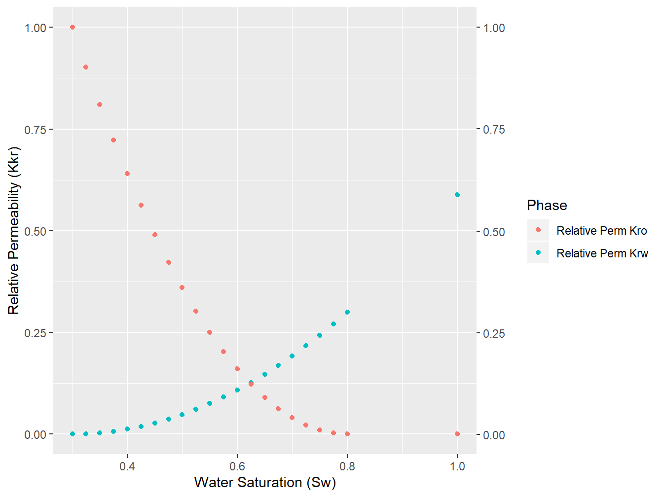
Figure 2.2: Relative Permeability Curves, water/oil System
2.2.2 Generating Geological Realization using Gaussian Sequential simulation (SGS)
In this work, Sequential Gaussian Simulation (SGS) was used to generate realizations of the each permeability. For example, in the 5-spot pattern, the permeability of the 5 wells (4 injectors and one producer) are driven randomly from the distribution of the permeability of the field which has the log-normal distribution.(Pyrcz and Deutsch 2014)
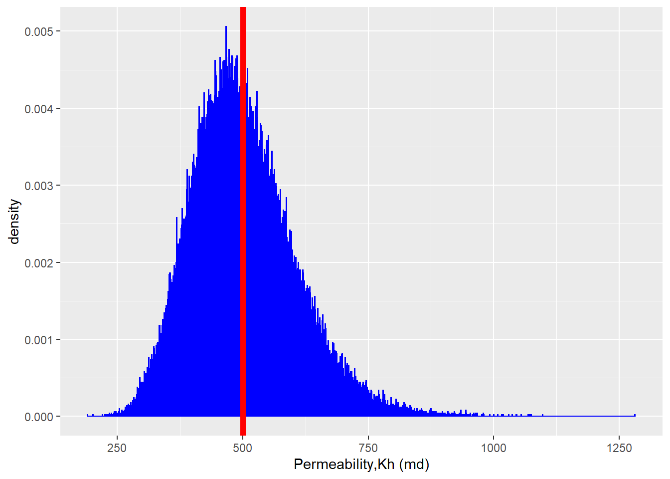
Figure 2.3: Log-Normal Distribution of the Field Permeability
For the sake of this work, we considered the following distribution in the Figure 2.3 as the distribution of the permeability in the field under study (It is considered \(K_{h}=K_{v}\))
Now, for every training observation [^2], we build 10 realizations [^3] of the permeability. SGS starts by creating a grid of randomly assigned values drawn from a standard normal distribution (mean = 0 and SD = 1). The co-variance model (from the semivariogram defined in the Simple Kriging layer, which is required as input for generating realizations ) is then applied. This ensures that raster values conform to the spatial coordinates found in the input data-set. The resulting raster constitutes one unconditional realization, and many more can be produced using a different raster of random values from gaussian Distribution at each time.
The steps involved in SGS can be summarized as the follows:
Step 1: In this case, the log 10 of permeability data are transformed into Gaussian values using the Q-Q plot.
Step 2: The distance matrix is calculated, that is the distance between the data and the unknown location. Here the unknown locations are the random path.
Step 3: Input the model of spatial continuity in the form of an isotropic spherical variogram and nugget effect (contributions should sum to one).
Step 4: Variogram matrix is calculated by applying the distance matrix to the isotropic variograms model.
Step 5: Covaraince matrix is calculated by subtracting the variogram from the variance (1 for standard normal distribution).
Step 6: The left hand side of the co-variance matrix is inverted.
Step 7: The inverted left hand-side matrix is multiplied by the right hand side matrix to calculate the simple kriging weights.
Step 8: The kriging estimate and kriging variance are calculated with the weights and co-variances.
Step 9: With the Gaussian assumption for the local CDF, the Monte Carlo simulation is applied to draw simulated realizations at the random path.
For example, for one of the training data set in five-spot pattern, the following permeability (in md) were drawn from the field permeability distribution (Figure 2.2). The X and Y shows spatial coordinates of the production well and injection wells, while the columns three and four provide the permeability value of those points.
| X | Y | Perm | logperm |
|---|---|---|---|
| 225 | 225 | 614.6815 | 2.788650 |
| 45 | 435 | 462.9789 | 2.665561 |
| 375 | 345 | 558.9657 | 2.747385 |
| 125 | 15 | 603.3033 | 2.780536 |
| 325 | 25 | 515.1680 | 2.711949 |
To visualize the data shown in the Table 2.2, the Figure 2.4 shows the spatial locations of the 5 points for calculating SGS. As was mentioned, the X and Y coordinates both has 45 grids with the size of the 10 m, therefore the coordination of the plot in Figure 2.4 will be from 0 to 450 m in both X and Y direction. It must be mentioned that in the all training data-set, we considered the production well is located in the center of geological model, in other word in grid (23,23).
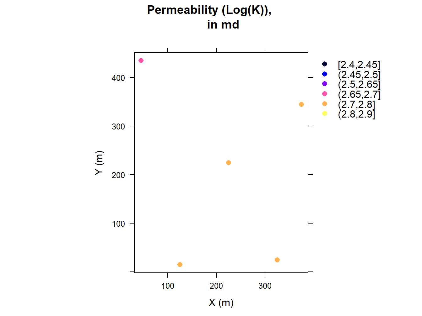
Figure 2.4: Graphical Representation of Five Permeability Points, Shown in the X, Y Coordinates
In this work the parameters of the semivariogram to generate different realization out of SGS method has been depicted in the Table 2.3. Note to mention that the sill considered for nugget effect is the the variance of the 5 permeability points in the Table 2.2.
| Parameter | Value |
|---|---|
| Nugget Effect | Sill/2, md^2 |
| Type | Spherical |
| Range | 20 (grid cell) |
| Anistropy ratio | 1 |
| Azimuth | 0-degree (North) |
Having specified the 5 permeability points and semivariogram parameters the SGS method could be performed. The Figure 2.5 shows the four realizations. In this work, every training observation has 10 permeability realizations.(Note, the range of color-bar at each realization in the Figure 2.5 starts from the minimum of the permeability until maximum of the permeability at THAT realization.)
## drawing 10 GLS realisations of beta...
## [using conditional Gaussian simulation]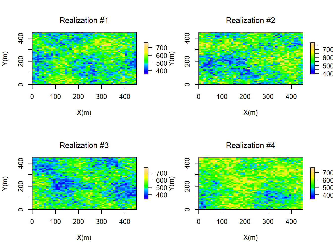
Figure 2.5: Four Realizations of the Permeability Ditribution Found Using SGS Method
2.2.3 Measure of Connectives
The FMM is a numerical method for the tracking the monotonically advancing surface on a grid based structure. One of the prorogation problem is where the prorogation waves moves in one direction and strictly expands. This boundary values equation is known as Eikonal equation and can be written as:
\[\begin{equation} F(x) |\bigtriangledown \tau(x)| = 1 \tag{2.1} \end{equation}\]
where the \(\tau\) is the arrival time , F is speed function. The FMM is introduced by (Sethian 1996) as numerical method for solving Equinal form of equation. The first-order fast-marching formulation to calculate the propagation time in each grid (\(\tau_{i,j,k}\)) can be summarized as:
\[\begin{equation} \mu c_t(x) \phi(x) \frac{\partial p(x,t)}{\partial t} -k(x)[\bigtriangledown ^{2} p(x,t)]-\bigtriangledown k(x).\bigtriangledown p(x,t) = 0 \tag{2.2} \end{equation}\]
where \(p(x)\) is the pressure, \(\phi(x)\) is the porosity, \(k(x)\) is the permeability, \(\mu\) is the viscosity , and \(c_t(x)\) is the total compressible (summation of rock and fluid compressibility). Using the Fourier transform , the Equation could be written as:
\[\begin{equation} \frac{\mu c_t \phi(x)}{k(x)} i w\hat{p}(x,w) - \frac{\bigtriangledown k(x)}{k (x)}.\bigtriangledown \hat{p}(x,w) -\bigtriangledown^2\hat{p}(x,w) = 0 \tag{2.3} \end{equation}\]
Assuming the heterogeneous media the \(\frac{\bigtriangledown k(x)}{k (x)}\) is negligible we can write:
\[\begin{equation} \bigtriangledown^2\hat{p}(x,w) - \frac{1}{\eta (x)} i w\hat{p}(x,w) = 0 \tag{2.4} \end{equation}\]
Where the term \(\eta (x) = \frac{k(x)}{\mu c_t \phi(x)}\) is called diffusivity.
An asympotic solution gives:
\[\begin{equation} \hat{p} (x,w) = e^{[-\sqrt{-iw} \tau(x)]} \sum_{n=0}^{\infty} \frac{A_n(x)}{(\sqrt{-iw})^n} \tag{2.5} \end{equation}\]
where the \(w\) is the frequency, \(\tau(x)\) is phase propagation, and \(A_n(x)\) is the coefficient of in the expansion. The previous equation can be used to calculate the operators:
\[\begin{equation} \bigtriangledown\hat{p}(x,w)=e^{[-\sqrt{-iw} \tau(x)]} \sum_{n=0}^{\infty} \frac{1}{(\sqrt{-iw})^n} \times[-\sqrt{-iw} A_n(x) \bigtriangledown \tau(x) +\bigtriangledown A_n(x)] \tag{2.6} \end{equation}\]
\[\begin{equation} \bigtriangledown^{2}\hat{p}(x,w)=e^{[-\sqrt{-iw} \tau(x)]} \sum_{n=0}^{\infty} \frac{1}{(\sqrt{-iw})^n} \times[-(\sqrt{-iw})^2 A_n(x) \\ \bigtriangledown \tau(x) \bigtriangledown\tau(x) -\sqrt{-iw}\bigtriangledown\tau(x) \\ \bigtriangledown A_n(x)-\sqrt{-iw} A_{n}(x) \bigtriangledown^2\tau(x)-\sqrt{-iw} \\ \tau(x)-\sqrt{-iw}\bigtriangledown A_n(x) \bigtriangledown \tau(x) +\bigtriangledown^2 A_n(x)] \tag{2.7} \end{equation}\]
\[\begin{equation} \bigtriangledown^{2}\hat{p}(x,w)=e^{[-\sqrt{-iw} \tau(x)]}\sum_{n=0}^{\infty} \\ \frac{1}{(\sqrt{-iw})^n} \times[-(\sqrt{-iw})^2 A_n(x) \bigtriangledown \tau(x) \\ \tag{2.8} \end{equation}\]
Now this equation can be written as:
\[\begin{equation} e^{[-\sqrt{-iw} \tau(x)]}\sum_{n=0}^{\infty} \frac{1}{(\sqrt{-iw})^{n-2}} \\ \times[A_{n}(x)\bigtriangledown \tau(x) \bigtriangledown \tau(x) -\frac{1}{\eta (x)} -2 \\ \bigtriangledown \tau(x) \bigtriangledown A_{n-1}(x) \tag{2.9} \end{equation}\]
one can set zero to the coefficient of the the individual powers of \(\sqrt{-iw}\) starting with the highest power \((\sqrt{-iw})^2\), now we can write:
\[\begin{equation} \bigtriangledown \tau(x) \bigtriangledown \tau(x) -\frac{1}{\eta (x)} = 0 \tag{2.10} \end{equation}\] The above equation has the Eikonal form and relates the \(\tau(x)\) we call it diffusive propagation time to \(\eta(x)\) which is the diffusivity coefficient.
\[\begin{equation} F(x) = \sqrt{\frac{k(x)}{\mu c_t(x) \phi(x) }} max(\frac{\tau-\tau_1}{\bigtriangleup x/F_I},0)^2 + max(\frac{\tau-\tau_2}{\bigtriangleup \\ /F_{J}},0)^2+max(\frac{\tau-\tau_3,}{\bigtriangleup z/F_{K}},0)^2 = 1 \tag{2.11} \end{equation}\]
2.2.4 Analytical Method
Now, in this section the goal is to compare results of the FMM method in tracking the pressure waves with the well known analytical well testing method. Considering the homogeneous reservoirs model with the characteristics depicted in the Table 2.4, the radius of investigation( Here, the radius of investigation is defined as the the radius, the pressure waves reaches after time (t)).
\[\begin{equation} r= \sqrt{\frac{kt}{948 \mu c_t \phi}} \tag{2.12} \end{equation}\]
Where t is the time (hours), k is the permeability (md), \(\mu\) is the viscosity (cp), \(c_t\) is the total compressibility (1/psi), and \(\phi\) is the porosity.
The figure plotted in Figure 2.6 shows the time pressure arrives at different radius (as contour plot). As could be seen, the FMM methods performs well in the capturing the pressure propagation compared to the exact analytical solution found from concept of the radius of investigation. However, the analytical method developed was valid in the case of the homogeneous reservoir model, whereas the geological model considered in this study is fully heterogeneous, therefore in he rest of this work, the FMM method will be used to calculate the connectivities between each pair point.
| Parameter | value |
|---|---|
| Grid-block Size | 20 by 20 by 20 |
| Porosity | 10% |
| Permeability | 1 md |
| Compressibility | 10^-5 |
| Viscosity | 1 cp |
| Initial pressure | 4000 psi |
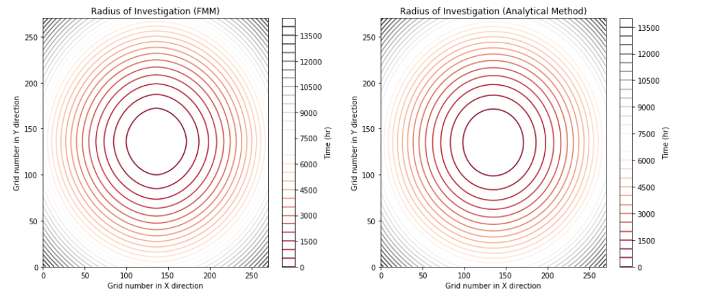
Figure 2.6: Comparison of Pressure Wave Propogation Profiles, FMM Method vs Analytical Solution
2.2.5 Features and Response
To utilize the Machine Learning method, we need to define the features of the model and as well response we are looking for. In this work the features of models are:
- Features
- Connectivity
- Pore Volume Flight
- Response
- NPV The connectivity is defined by the value of ‘diffusive time of flight’ and the PV is the defined as the sum of all grid affected by pressure disturbance when the pressure propagation reach the injection well.
The NPV is defined as the below:
\[\begin{equation} NPV=\sum_{k=1}^{n_T} \frac{[q_o^{k}P_o - q_w^k P_w -I^k P_{wi} ]\bigtriangleup t_k}{(1+b)^{t_k/D}} \tag{2.13} \end{equation}\]
Where the parameter is defined is below: \(q_o^{k}\): is the field oil production rate at time k \(q_w^{k}\): is the field water production rate at time k \(I^k\): is the field water injection rate at time k \(P_o\): is the oil price \(P_wp\): is the water production cost \(P_wi\): is the water injection cost \(b\): is the discount factor \(t-k\): is the cumulative time for discounting \(D\): is the reference time for discounting (D=365 days if \(b\) is expressed as fraction per year and the cash flow is discounted daily) \(q_o^k\),\(q_w^k\) and \(I^k\) are forecasted by given production model.
In this work, the following economical parameters were considered to calculate the Net Present Value after recessing the Numerical Reservoir Simulator.
| Parameter | value |
|---|---|
| Oil Price, per barrel | 70 $ |
| Water Production Cost, per barrel | 15$ |
| Water Injection Cost, per barrel | 5$ |
| Discount Factor | 8% |
2.2.6 Machine Learning Algorithm
Big data vary in These call for different approaches. Wide data consists of :
Thousands/Millions of variables Hundreds of samples
Tall data has a dimension in the following range:
Tens/Hundreds of Variables Thousands/ Millions of Samples
In briefly, the most well-known ML algorithm can be summarized as the follows:
- Linear/Logistics Regression
- k-Nearest Neighbours
- Support Vector Machine
- Tree-based Model Decision Tree Random Forest Gradient Boosting Machine Neural Networks
In this work, We use the XGBoost (short for extreme Gradient Boosting) ML model since it has showed several successful application in oil and gas industry and as well is the winning model for several Kaggle competitions (A. Nwachukwu, Jeong, Pyrcz, et al. 2018, @nwachukwu2019machine).
2.2.7 eXtreme Gradient Boosting Model
suppose we have K trees, the model is defined as:
\[\begin{equation} \sum_{k=1}^{K} f_k \tag{2.14} \end{equation}\]
Where each \(f_k\) is the prediction from a decision tree . The model is a collection of decision trees. Having all the decision trees, we make prediction by:
\[\begin{equation} \hat{y}_i = \sum_{k=1}^{K}f_k(x_i) \tag{2.15} \end{equation}\]
where \(x_i\) is the feature vector for the \(i-th\) data point. Similarly , the prediction at the\(t-th\) step can be defined as:
\[\begin{equation} \hat{y}_{i}^{(t)}=\sum_{k=1}^{t} f_k(x_i) \tag{2.16} \end{equation}\]
To train the model, the loss function need to be optimized:
- Rooted Mean Square Error for regression
\[L = \frac{1}{N}\sum_{i=1}^{N}(y_i - \hat{y}_i)^2\]
- Log- Likelihood for multi-classification
\[ L = -\frac{1}{N}\sum_{i=1}^{N}\sum_{j=1}^{M} y_{i,j} log(p_{i,j})\]
Regularization is another important part of the model. A good regularization term controls the complexity of the model which prevents over- fitting.
\[\begin{equation} \Omega = \gamma T + \frac{1}{2} \gamma \sum_{j=1}{T}w_j^2 \tag{2.17} \end{equation}\]
Where T is the number of the leaves, and \(w_j^2\) is the score on the j-th leaf. Putting loss function and regularization together, we have the objective of the model: \[Obj = L +\Omega\] In the XGBoost method, the gradient descent is used to optimize the objective. Given an objective \(Obj(y, \hat{y})\) to optimize, gradient descent is an iterative technique which calculate:
\[\begin{equation} \partial_{\hat{y}} Obj(y,\hat{y}) \tag{2.18} \end{equation}\]
at each iteration.Then we improve \(\hat{y}\) along the direction of the gradient to minimize the objective. In the case of iteration, the Objective function \(Obj = L+\Omega\) can be defined as :
\[\begin{equation} Obj^{(t)}=\sum_{i=1}^{N} L(y_i,\hat{y}_i^{(t)}) +\sum_{i=1}^{t} \Omega(f_i) = \sum_{i=1}^{N} L(y_i,\hat{y}^{(t-1)} + f_t(x-i))+\sum_{i=1}^{t} \Omega(f_i) \tag{2.19} \end{equation}\]
The tree structure in XGBoost leads to the core problem: How we can find a tree that improves the prediction along the gradient? The idea of the gradient descent is used to solve this problem.
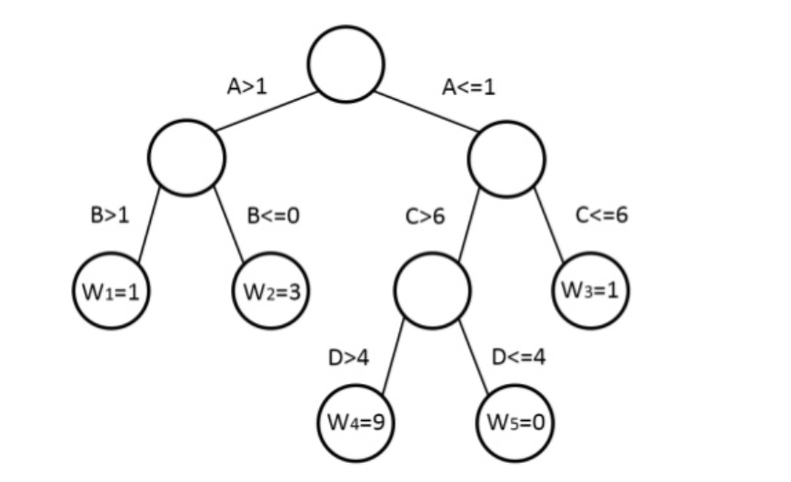
Figure 2.7: Representation of a Decision Tree in XGBOOST
2.2.8 Model Building and Validation
In this, 500 training observation were used to build the ML model. Each training observation then has 10 realizations that make total training data set equal to 5000. The features of this model has been shown in the table.
| Parameter |
|---|
| Connectivity Pair (Inj1-Inj2) |
| Connectivity Pair (Inj3-Inj1) |
| Connectivity Pair (Inj3-Inj2) |
| Connectivity Pair (Inj4-Inj1) |
| Connectivity Pair (Inj4-Inj2) |
| Connectivity Pair (Inj4-Inj3) |
| Connectivity Pair (Pro1-Inj1) |
| Connectivity Pair (Pro1-Inj2) |
| Connectivity Pair (Pro1-Inj3) |
| Connectivity Pair (Pro1-Inj4) |
| PV of Flight |
Then, the Table 2.6 provides the features that carries the information about the geology and pressure propagation in the reservoir model, not the injection rate parameters. To include the injection scenarios, the exponential form of injection scenario was considered, as the follow:
\[\begin{equation} A*exp(-\gamma*t) \tag{2.20} \end{equation}\]
Here, we consider the 5 different \(A\) values as the starting injection rates and 11 \(\gamma\). Therefore, the total injection scenario included in this work is (\(5*11=55\)). In the Figure 2.8 we can see the 55 injection scenarios having 11 values for \(\gamma\) (left side of the Figure) and Showing all scenarios (Right side of the figure).
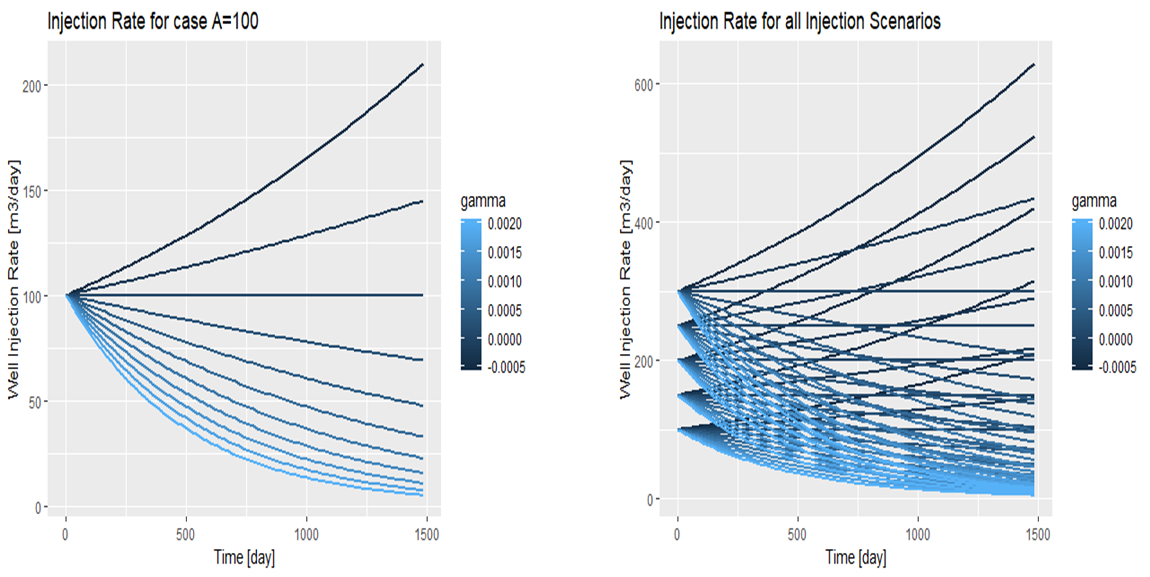
Figure 2.8: Left: 11 Injection Scenarios at A=100, Right: All Injection Schemes
Now, specifying each injection scenarios based on it’s \(A\) and \(\gamma\) values, we can theses features to our initial features, to complete the features which captures both the physic of the flow and the control parameters.
| Features |
|---|
| Connectivity Pair (Inj1-Inj2) |
| Connectivity Pair (Inj3-Inj1) |
| Connectivity Pair (Inj3-Inj2) |
| Connectivity Pair (Inj4-Inj1) |
| Connectivity Pair (Inj4-Inj2) |
| Connectivity Pair (Inj4-Inj3) |
| Connectivity Pair (Pro1-Inj1) |
| Connectivity Pair (Pro1-Inj2) |
| Connectivity Pair (Pro1-Inj3) |
| Connectivity Pair (Pro1-Inj4) |
| PV of Flight |
| A value for Inje1 |
| A value for Inj2 |
| A value for Inj3 |
| A value for Inj4 |
| Gamma value for Inj1 |
| Gamma value for Inj2 |
| Gamma value for Inj3 |
| Gamma value for Inj4 |
Now, the full sets of the features shown in the Table 2.7 and the output of the ML (NPV) is ready. The number of training data set is (N=5000) and the algorithm of ML is XGBOOST. The ML algorithm here has six parameter that needed to be tuned. Therefore, hyper parameter optimization process was doe considering 288 combination of the parameters to fund the tuned parameters of the ML. It must be mentioned that, in this work 5-fold Cross- validation was used to avoid any potential over-fitting problem in the development of the ML. The final parameters of the ML in this work can be shown in the Figure 2.8
| XGBOOST Parameter | Value |
|---|---|
| nrounds | 4000 |
| Max_depth | 6 |
| Etta | 0.001 |
| Gamma | 0 |
| Min_Child_Weight | 2.25 |
| Sub-sample | 1 |
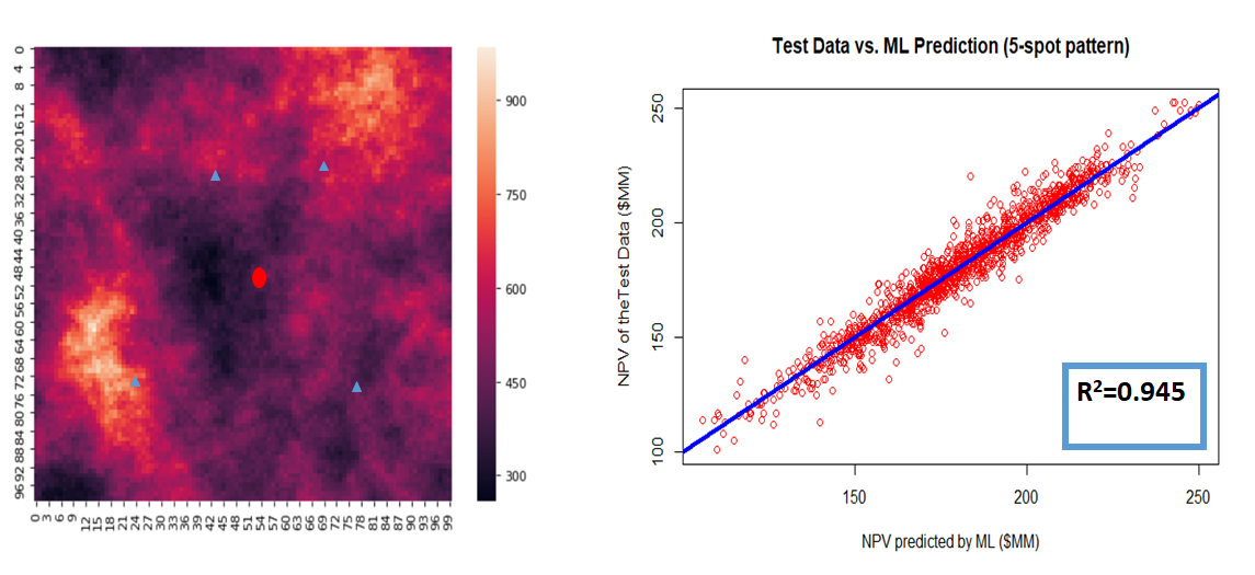
Figure 2.9: An Example of a Training Data Set and Testing Model Capability
[^1] Here, we call proxy reservoir model because it is less rich in complexity and in addition is not fully based on solving governing physical equations, rather model reduced form of the physical models. [^2]: In this work training observation means the same geological model which has the different well locations and injection scenarios. [^3]: The realization in this work means the same well placement and and injection rates but different permeability distribution to capture the uncertainty of this petrophysical parameter.
References
Ahmadi, Mohammad Ali, Mohammad Ebadi, Amin Shokrollahi, and Seyed Mohammad Javad Majidi. 2013. “Evolving Artificial Neural Network and Imperialist Competitive Algorithm for Prediction Oil Flow Rate of the Reservoir.” Applied Soft Computing 13 (2). Elsevier: 1085–98.
Box, George EP. 1979. “All Models Are Wrong, but Some Are Useful.” Robustness in Statistics 202.
Bratvold, Reidar B, J Eric Bickel, Hans Petter Lohne, and others. 2009. “Value of Information in the Oil and Gas Industry: Past, Present, and Future.” SPE Reservoir Evaluation & Engineering 12 (04). Society of Petroleum Engineers: 630–38.
Castelletti, A, Stefano Galelli, Marcello Restelli, and Rodolfo Soncini-Sessa. 2010. “Tree-Based Reinforcement Learning for Optimal Water Reservoir Operation.” Water Resources Research 46 (9). Wiley Online Library.
Nwachukwu, Azor, Hoonyoung Jeong, Michael Pyrcz, and Larry W Lake. 2018. “Fast Evaluation of Well Placements in Heterogeneous Reservoir Models Using Machine Learning.” Journal of Petroleum Science and Engineering 163. Elsevier: 463–75.
Pyrcz, Michael J, and Clayton V Deutsch. 2014. Geostatistical Reservoir Modeling. Oxford university press.
Sayarpour, Morteza, C Shah Kabir, Larry W Lake, and others. 2009. “Field Applications of Capacitance-Resistance Models in Waterfloods.” SPE Reservoir Evaluation & Engineering 12 (06). Society of Petroleum Engineers: 853–64.
Sethian, James A. 1996. “A Fast Marching Level Set Method for Monotonically Advancing Fronts.” Proceedings of the National Academy of Sciences 93 (4). National Acad Sciences: 1591–5.
Sharifi, Mohammad, Mohan Kelkar, Asnul Bahar, Tormod Slettebo, and others. 2014. “Dynamic Ranking of Multiple Realizations by Use of the Fast-Marching Method.” SPE Journal 19 (06). Society of Petroleum Engineers: 1–069.
Stalgorova, Ekaterina, Tayfun Babadagli, and others. 2012. “Field-Scale Modeling of Tracer Injection in Naturally Fractured Reservoirs Using the Random-Walk Particle-Tracking Simulation.” SPE Journal 17 (02). Society of Petroleum Engineers: 580–92.
Yu, Shiwei, Kejun Zhu, and Fengqin Diao. 2008. “A Dynamic All Parameters Adaptive Bp Neural Networks Model and Its Application on Oil Reservoir Prediction.” Applied Mathematics and Computation 195 (1). Elsevier: 66–75.