Chapter 15 Normal distribution
Motivating scenarios: We want to understand what’s so special about the normal distribution – what are its properties? Why do we see it so often? Why di we use it so often? What is it good for?….
Learning goals: By the end of this chapter you should be able to
- Describe the properties of a normal distribution.
- Know that the standard error of the sampling distribution of size n from the normal distribution equals \(\frac{\sigma}{\sqrt{n}}\).
- Find the probability density of a (range of) sample mean(s).
- Use a Z-transform to convert any normal distribution into the standard normal distribution.
- Interpret histograms and qq-plots to meaningfully evaluate if data are roughly normal.
- Explain why normal distributions are common, and explain the Central Limit Theorem.
- Transform non normal data to become normal
- Use the
_norm()family of functions to- simulate random numbers from a normal distribution (
rnorm()).
- Calculate the probability density of an observation from a specified normal distribution (
dnorm()).
- Calculate the probability of finding a value more extreme than some number of interest from a specified normal distribution
pnorm(), and
- Find a specified quantile of a normal distribution with
qnorm()).
- simulate random numbers from a normal distribution (
15.1 Probability densities for continuous variables.
The binomial distribution (Chapter ??) is a discrete distribution – we can write down every possible outcome (zero success, one success, etc… n successes) and calculate its probability. Adding these up will sum to one (i.e. \(\sum p_x=1\)). Probabilities of these possible outcomes (those which sum to one within discrete distributions) are called probability masses. E.g. the probability of heads on a coin toss is called its probability mass.
By contrast, the probability of any one outcome from a continuous distribution, like the normal distribution, is infinitesimally small because there are infinite numbers in any range. We therefore describe continuous distributions with probability densities. Probability densities integrate to one (i.e. \(\int p_x=1\)), and can therefore even exceed one for some points. (e.g. Fig 15.1)
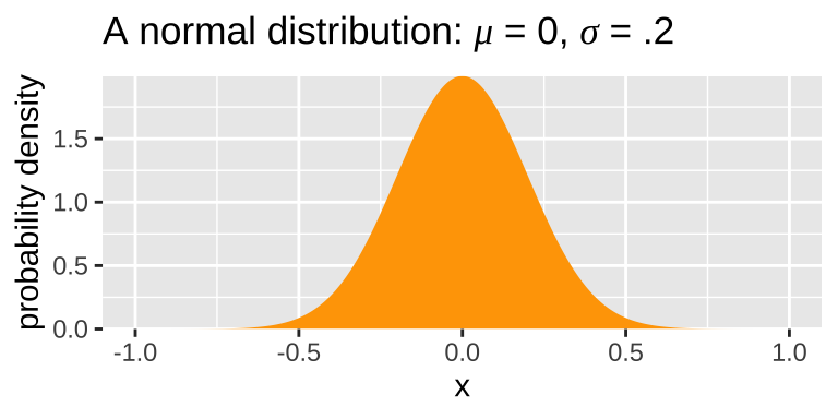
Figure 15.1: A normal distribution with a mean of one and standard deviation of 0.2.
15.2 The many normal distributions
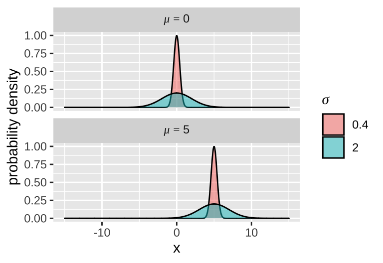
Each normal distribution is fully characterized by two parameters – a mean \(\mu\), and variance \(\sigma^2\) (or standard deviation, \(\sigma\)). I show four different normal distributions – all combinations of \(\mu =0\) or \(\mu = 5\), and \(\sigma = 2\) or \(\sigma = .2\) to the right.
The probability density for each value on the x equals You do not need to know this.
\[\begin{equation} f(x)={\frac {1}{\sigma {\sqrt {2\pi }}}}e^{-{\frac {1}{2}}\left({\frac {x-\mu }{\sigma }}\right)^{2}} \tag{15.1} \end{equation}\]
We efficiently describe a normally distributed random variable as \(X \sim N(\mu,\sigma^2)\), where \(\sim\) means is distributed. So, the mathematical notation to say \(X\) is normally distributed with mean \(\mu = 0.5\) and variance \(\sigma^2 = 0.1^2\) is \(X \sim N(0.5,0.01)\).
15.2.1 Using R to claculate a probability density
Like the dbinom() function calculates the probability of a given observation from a binomial distribution by doing the math of the binomial distribution for us, dnorm() calculates the probability density of an observation from a normal distribution by plugging and chugging through Equation (15.1).
For example, dnorm(x = .4, mean = .5, sd = .1) goes through Eq. (15.1), plugging in \(0.4\) for \(x\), \(0.5\) for \(\mu\), and \(0.1\) for \(\sigma\) to return 2.42.
15.2.2 The probability density of a sample mean
Remember that the standard deviation of the sampling distribution is called the standard error. It turns out that the standard error of a sample of size n from the normal distribution equals \(\frac{\sigma}{\sqrt{n}}\).
So, we get probability density of a sample mean by substituting \(\sigma\) in Equation (15.1) with the standard error \(\frac{\sigma}{\sqrt{n}}\). Therefore, while the probability density that a random draw from a normal distribution with \(\mu =0.5\) and \(\sigma = 0.1\) equals 0.4 is dnorm(x = .4, mean = .5, sd = .1) = 2.42.
By contrast the probability density that the mean of a sample size 25 from the distribution equals 0.4 is
dnorm(x = .4, mean = .5, sd = .1 / sqrt(25))
- =
dnorm(x = .4, mean = .5, sd = .02)
- = \(7.43 \times 10^{-5}\)
15.2.3 The standard normal distribution and the Z transform
The most famous normal distribution, the “standard normal distribution” (aka Z*, has a mean of zero and a standard deviation of one. That is, \(X \sim N(0,1)\).
Any normal distribution can be converted to the standard normal distribution by subtracting the population mean, \(\mu\), from each value and dividing by the population standard deviation, \(\sigma\) (aka the Z transform).
\[Z=\frac{X-\mu }{\sigma }\] So, for example, by a Z transform, a value of \(X=0.4\) from a normal distribution with \(\mu = 0.5\) and \(\sigma = 0.1\), will be \(\frac{0.4 -0.5}{0.1} = \frac{-0.1}{0.1} = -1\).
15.3 Properties of a normal distribution
15.3.1 A Normal Distribution is symmetric about its mean
This means
- That half of the normal distribution is greater than its mean and half is less that its mean. For example if \(X \sim N(.5, .1^2)\),
pnorm(q = 0.5, mean = 0.5, sd = 0.1, lower.tail = TRUE)
- =
pnorm(q = 0.5, mean = 0.5, sd = 0.1, lower.tail = FALSE)
- = 0.5.
- The probability density of being some distance away from the true mean is equal regardless of direction. For example:
dnorm(x = 0.4, mean = 0.5, sd = 0.1)
- =
dnorm(x = 0.6, mean = 0.5, sd = 0.1)
- = 2.4197.
- The probability of being some distance away from the true mean or more extreme is equal regardless of if you’re that much less than (or more) or that much greater than the mean (or more). For example:
pnorm(q = 0.4, mean = 0.5, sd = 0.1, lower.tail = TRUE)
- =
pnorm(q = 0.6, mean = 0.5, sd = 0.1, lower.tail = FALSE)
- = 0.1587.
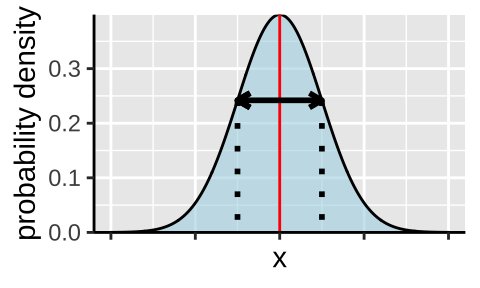
15.3.2 Probability that X falls in a range
The probability that x lies between two values, \(a\) and \(b\) is \[P[a <X < b] = \int_{a}^{b} \frac{1}{\sqrt{2\pi \sigma ^{2}}}e^{-\frac{(x-\mu) ^{2}}{2\sigma ^{2}}} dx\]
Some helpful (approximate) ranges:
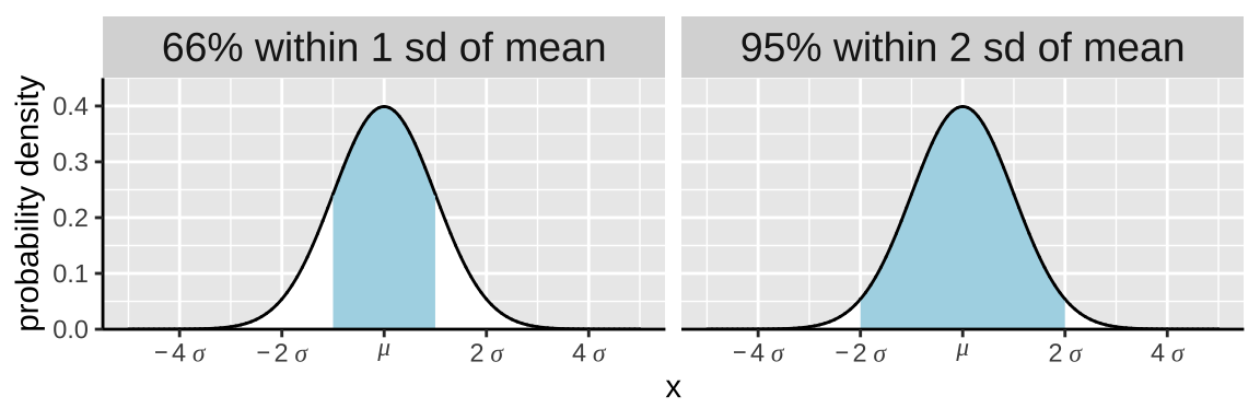
More exactly, the probability that X is within one standard deviation away from the mean equals
- The probability it is not more than one standard deviation less than its mean
pnorm(q = -1, mean = 0, sd = 1, lower.tail = FALSE)
- = 0.8413
- Minus the probability it is not more than one standard deviation greater than its mean
pnorm(q = 1, mean = 0, sd = 1, lower.tail = FALSE)
- = 0.1587.
- Which equals
0.841 - 0.158
- =
0.683
For this example we used the standard normal distribution for ease, but this is true for any normal distribution… e.g. pnorm(q = 10, mean = 5, sd = 5, lower.tail = FALSE) = 0.1587.
15.3.2.1 Probability that a mean, \(\overline{X}\), falls in a range
Again, we can take advantage of the fact that the standard deviation of a sampling distribution is the standard error divided by the square root of the sample size. So the probability that a mean, \(\overline{X}\) lies between two values, \(a\) and \(b\) is \[P[a < \overline{X} < b] = \int_{a}^{b} \frac{1}{\sqrt{2\pi \sigma ^{2}/n}}e^{-\frac{(x-\mu) ^{2}}{2\sigma ^{2}/n}} dx\].
So, for example, the probability that the mean of four draws from the standard normal distribution is between -1 and 1 is
- The probablity is is greater than negative one
pnorm(q = -1, mean = 0, sd = 1/sqrt(4), lower.tail = FALSE)
rpnorm(q = -1, mean = 0, sd = 1/sqrt(4), lower.tail = FALSE) %>% round(digits = 4)`
- Minus the probablity is greater than one
pnorm(q = 1, mean = 0, sd = 1/sqrt(4), lower.tail =FALSE)
- 0.0228
- Equals \(0.977 - 0.022 = 0.955\)
Let’s prove this to ourselves by generating four random numbers from the standard normal distribution many times using rnorm()
# set up
n_reps      <- 100000
sample_size <- 4
this_mean   <- 0
this_sd     <- 1

tibble(sample = rep(1:n_reps, each = sample_size),
       value  = rnorm(n = n_reps * sample_size, mean = this_mean, sd = this_sd)) %>%
  group_by(sample)                              %>%
  summarise(mean_x          = mean(value))      %>%
  mutate(within_one         = abs(mean_x) < 1 ) %>%
  summarise(prop_within_one = mean(within_one))
## # A tibble: 1 × 1
## prop_within_one
## <dbl>
## 1 0.954
15.3.3 Quantiles of a Normal Distribution
Above, I said that about 95% of samples are within two standard deviations of a normal distribution. That is a close approximation. Like our work above, we can find the proportion of samples within two standard deviations of the mean as pnorm(q = 2, mean = 0, sd =1) - pnorm(q = -2, mean = 0, sd =1) = 0.9544997.
But say we wanted to reverse this question, and find the values that separate the middle 95% of samples from the extremes (i.e. the critical values at \(\alpha = 0.05\)). The [qnorm()] function (where q is for quantile) is here for us. We find a two tailed critical value as qnorm(p = 1 - alpha/2, mean = 0, sd = 1), where \(\alpha\) is our specified alpha value and we divide by two because we’re considering an equal area on both tails. So 95% of samples (of size one) from a normal distribution are within qnorm(p = 1 - 0.05/2, mean = 0, sd = 1) = 1.96 standard deviations of the mean.
15.4 Is it normal
Much of the stats we will learn soon relies, to some extent, on the normal data (or more specifically, a normally distributed sampling distribution of residuals). While there are statistical procedures to test the null hypothesis that data come from a normal distribution, we almost never use these because a deviation from a normal distribution can be most important when we have the least power to detect it. For that reason,we usually use our eyes, rather than null hypothesis significance testing to see if data are approximately normal
15.4.1 “Quantile-Quantile” plots and the eye test
In a “quantile-quantile” (or QQ) plot x is y’s z-transformed expectation i.e. mutate(data, qval = rank(y)/(n+.5), x = qnorm(qval)), and y is the data. Data from a normal distribution should fall near a straight line.
In R We can make a qq-plot with the geom_qq() function and add a line with geom_qq_line(), here we map our quantity of interest onto the attribute, sample. As an example, I present a qq-plot of petal lengths in Iris versicolor in Figure 15.2.
iris %>%
  filter(Species == "versicolor") %>%
  ggplot( aes(sample = Petal.Length))+
  geom_qq()+
  geom_qq_line()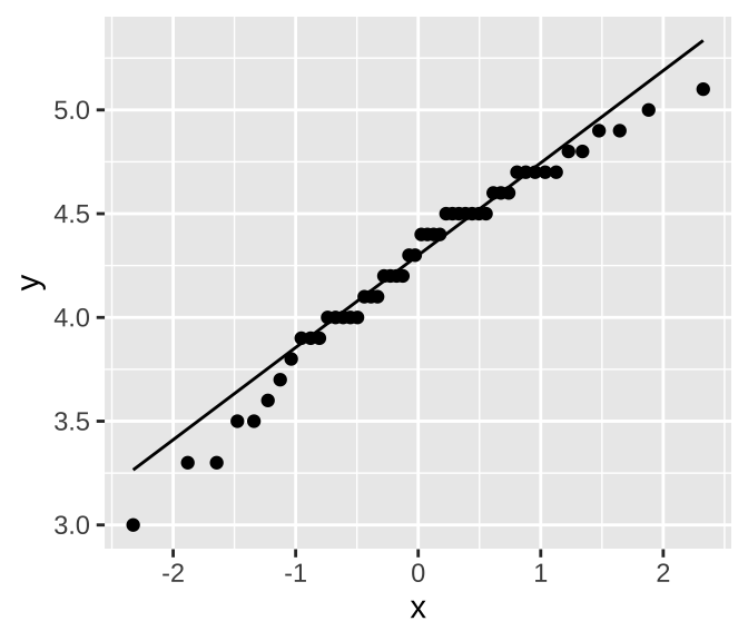
Figure 15.2: A quantile quantile plot of Petal Length in Iris versicolor.
We can see that points seem to be pretty close to the predicted line, but both the small values and large values are a bit smaller than we expect. Is this a big deal? Is this deviation surprising? To find out we need to get a sense of the variability we expect from a normal distribution.
15.4.2 What normal distributions look like
I am always surprised about how easily I can convince myself that a sample does not come from a normal distribution. To give you a sense
Figure 15.3: Run this about ten times for five quite different sample sizes to get a sense for the variability in how normal a sample from the normal distribution looks. This basically takes your sample size, n, and simulates random data from the standard normal by running this R code my_dat <- tibble(x = rnorm(n = n, mean = 0, sd = 1)), and then plotting the output
15.4.3 Examples of a sample not from a normal distribution
Let’s compare the samples from a normal distribution, in Figure 15.3 to cases in which the data are not normal. For example,
- Figure 15.4 makes it clear that across the three Iris species, sepal length is bimodal.
- Figure 15.5 makes it clear that across all mammals the distribution of body weights are exponentially distributed.
These examples are a bit extreme. Over the term, we’ll get practice in visually assessing if data are normallish.
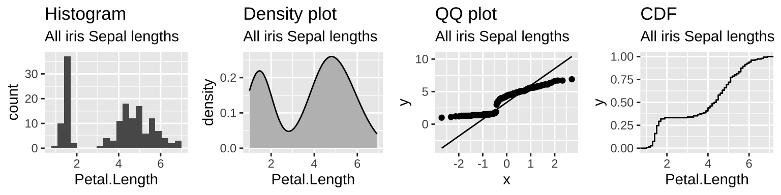
Figure 15.4: The distribution of petal lengths across all three iris species is bimodal – as the extremely small petals of iris setosa.
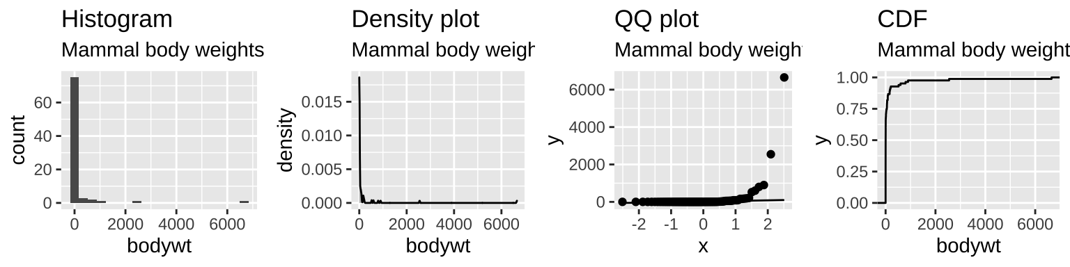
Figure 15.5: The distribution of mammal body size is exponentially distributed.
15.5 Why normal distributions are common
One amazing thing about the world is just how common the normal distribution is. The reason for this is that whenever a value comes from adding up a MANY INDEPENDENT things, this value will be normally distributed, regardless of the underlying distribution of these underling things. For example, your height is the result of the action of the many genes in your genome that influence it, the many environmental factors that influenced it … etc…
An important consequence of this is that the sampling distribution of means tends to be normally distributed, so long as the sample size isn’t too small. This rule, called the Central Limit Theorem is very useful for statistics because it means that we can make reasonable statistical models of sample means by assuming a normal distribution even if the underlying data points come from a distribution that isn’t quite normal.
15.5.1 How large must a sample be for us to trust the Central Limit theorem?
The central limit theorem assures us that, with a sufficiently ample sample size, the sampling distribution of means will be normal, regardless of the distribution of the underlying data points.
But how large is sufficiently large? The answer depends on how far from normal the initial data are. The less normal the initial data, the larger the sample size before the sampling distribution becomes normal.
Figure 15.6: The sampling distribution of a sample of size, sample size, from a few different distributions. A sample of size one corresponds to the raw data, while all other sample sizes show a sampling distribution. For each distribution, explore how many samples we need before the sampling distribution looks normal.
15.6 Transforming data
Because the normal distribution is so common, and because the central limit theorem is so useful, there are a bunch of statistical approaches made for data with some form of normality assumption. But sometimes data are too far from normal to be modeled as if they are normal. Other times, details of a statistical distribution lead to breaking other assumptions of statistical tests. When this happens, we have a few options.
- We can permute and bootstrap!!
- We can use/develop tools to model the data as they are actually distributed.
- We can transform the data to meet our assumptions.
We have already discussed option 1 at length, and will return to option 3 later in the term.
15.6.1 Rules for legit transformations
There is nothing “natural” about linear scale, so there is nothing wrong about transforming data to a different scale. In fact, we should estimate & test hypotheses on a meaningful scale. In fact an appropriate transformation will often result in normal-ish distributed data.
Rules for transforming data
- Let biology guide you. Often you can think through what transformation is appropriate by thinking about a mathematical model describing your data. So, for example, if values naturally grow exponentially, you should probably log-transform your data.
- Apply the same transformation to each individual.
- Transformed values must have one-to-one correspondence to original values. e.g. don’t square if some values are \(<0\) and some are \(>0\).
- Transformed values must have a monotonic relationship with the original values e.g., larger values stay larger, so be careful with trigonometric transformations.
- Conduct your statistical tests AFTER you settle on the appropriate transformation.
- Do not bias your results by losing data points when transforming the data.
15.6.2 Common transformations
There are numerous common transformations that will make data normal, depending on their initial shape.
| Name | Formula | What type of data? |
|---|---|---|
| Log | \(Y'=\log_x(Y + \epsilon)\) | Right skewed |
| Square-root | \(Y'=\sqrt{Y+1/2}\) | Right skewed |
| Reciprocal | \(Y'=1/Y\) | Right skewed |
| Arcsine | \(\displaystyle p'=arcsin[\sqrt{p}]\) | Proportions |
| Square | \(Y'=Y^2\) | Left skewed |
| Exponential | \(\displaystyle Y'=e^Y\) | Left skewed |
Transformation example: The log transformation
We have seen that the normal distribution arises when we add up a bunch of things. If we multiply a bunch of things, we get an exponential distribution. Because adding logs is like multiplying untransformed data, a log transform makes exponential data look normal.
Take our distribution of mammal body weights, for example. It is initially far from normal (Fig. 15.7A,C), but after a log transformation it is much closer to normal (Fig. 15.7B,D) and would likely have a normal sampling distribution for relatively modest sample sizes.
# log10 transform
msleep <-  mutate(msleep, log10_bodywt = log10(bodywt))

# let's evaluate normality
plot_grid(
  ggplot(msleep, aes(x = bodywt))            + geom_histogram() + labs(title = "Raw body weight"),
  ggplot(msleep, aes(x = log10_bodywt))      + geom_histogram() + labs(title = "log10(body weight)") ,
  ggplot(msleep, aes(sample = bodywt))       + geom_qq()        + geom_qq_line() ,
  ggplot(msleep, aes(sample = log10_bodywt)) + geom_qq()        + geom_qq_line() ,
  ncol =2, labels = "AUTO", rel_heights = c(5,4.5))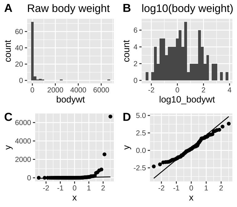
Figure 15.7: The mammal body mass data is very far from normal as seen in the histogram (A) and qq-plot (C). After log_10 transformation, data are much closer to normal (B and D). log_10 was chosen over the natural log because it is easier for most readers to interpret
log1p transform, which adds one to each number before logging them.
15.7 Log Likelihood of \(\mu\)
We have seen that calculating likelihoods is the basis for both maximum likelihood and Bayesian inference. How can we calculate likelihoods for a parameter of a normal distribution? Here’s how!
Say we had a sample with values 0.01, 0.07, and 2.2, and we knew the population standard deviation equaled one, but we didn’t know the population mean. We could find the likelihood of a proposed mean by multiplying the probability of each observation, given the proposed mean. So the likelihood of \(\mu = 0 | \sigma = 1, \text{ and } Data = \{0.01, 0.07, 2.2\}\) is
dnorm(x = 0.01, mean = 0, sd = 1) * dnorm(x = 0.07, mean = 0, sd = 1) * dnorm(x = 2.20, mean = 0, sd = 1)## [1] 0.00563186A more compact way to write this is dnorm(x = c(0.01, 0.07, 2.20), mean = 0, sd = 1) %>% prod(). Remember we multiply because all observations are independent.
For both mathematical and logistical (computers have trouble with very small numbers) reasons, it is usually better to work wit log likelihoods than linear likelihoods. Because multiplying on linear scale is like adding on log scale, the log likelihood for this case is dnorm(x = c(0.01, 0.07, 2.20), mean = 0, sd = 1, log = TRUE) %>% sum() = -5.1793156. Reassuringly, log(0.00563186) = -5.1793155.
We can find a likelihood profile as
obs            <- c(0.01, 0.07, 2.2)
proposed.means <- seq(-1, 2, .001)
tibble(proposed_means = rep(proposed.means , each = length(obs)),
       observations   = rep(obs, times = length(proposed.means)),
       log_liks       = dnorm(x = observations, mean = proposed_means, sd = 1, log = TRUE)) %>%
  group_by(proposed_means) %>%
  summarise(logLik = sum(log_liks)) %>%
  ggplot(aes(x = proposed_means, y = logLik))+
  geom_line()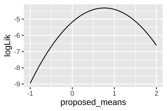
We can find the maximum likelihood estimate as
tibble(proposed_means = rep(proposed.means , each = length(obs)),
       observations   = rep(obs, times = length(proposed.means)),
       log_liks       = dnorm(x = observations, mean = proposed_means, sd = 1, log = TRUE)) %>%
  group_by(proposed_means) %>%
  summarise(logLik = sum(log_liks)) %>%
  filter(logLik == max(logLik)) %>%
  pull(proposed_means)
## [1] 0.76Which equals the mean of our observations mean(c(0.01, 0.07, 2.2)) = 0.76. More broadly, for normally distributed data, the maximum likelihood estimate of a population mean is the sample mean.