BLOCK 6: Dynamic Analysis

Class 1: Introduction to Difference Equations

What are these models necessary for?

For the first time we are going to deal in an explicit way with the variable time in the models. The idea of a model being dynamic (i.e. it includes the time variable) is for us to be able to to introduce trend concepts or cycles into the behavior of the variables. And in Economics it is a key, since the trend and the cycle are very appreciable behaviors in almost all economic and social variables.

So, these models may be very useful in trying to predict. PREDICT! The goal of science. Next to nothing.

An initial idea

Surely you have found many times in social networks challenges such as:

Follow the sequence: \[ 2,4,3,... \]

and, of course, one may think that there are many options to continue it. One way to work on any problem is to establish a model by hypothesis. Once you have the model, you fit it to the data and, if it works with the information you have, you try to PREDICT, which is what this exercise is all about.

Let’s imagine that the next value of the sequence depends on the previous one. For example, to “formalize” things somewhat, let’s say that the series of numbers will be called $x$ and the subscript will indicate the number of order of values. So, we have: \[ x_{0}=2,x_{1}=4,x_{2}=3 \]

and we would like to know $x_{3},x_{4},...,$ etc.

Our hypothesis is going to be that the “new” value will depend on the previous. To start with a simple model, let’s choose a linear equation:

\[ x_{new}=ax_{old}+b \]

In this way, we will have to

\[ \begin{cases} x_{1}=ax_{0}+b\\ x_{2}=ax_{1}+b \end{cases} \]

and substituting the values we know:

\[ \begin{cases} 4=a2+b\\ 3=a4+b \end{cases} \]

where we have a system (compatible determined) where $a = -1/2$ and $b=5$. Since these parameters make the system compatible with the data, we will say that we have a model that explains our available data. We can, then, use to generalize the behavior of this data sequence:

\[ x_{t+1}=-\frac{1}{2}x_{t}+5 \]

Where $t=0,1,2,3,....$ So, if we try to predict where the sequence will go, knowing that $x_{2}=3,$

\[ x_{4}=-\frac{1}{2}x_{3}+5\Rightarrow x_{4}=-\frac{3}{2}+5=3.5 \]

Another example: a piggy bank

Let’s imagine that in our current account we introduce every week 10 euros. Then, the variable “time” will be the weeks and the “initial” will be called “week zero.” Then, our account will look like this:

t		income balance
0	10	10
1	10	20
2	10	30
…	…	…
T	10	$(T-1)\times 10$

if we want to write these accounting operations using an equation, this could be:

\[ x_{t+1}=x_{t}+10 \]

That is, $x$ is the amount of money. This equation can be read how:

The money I will have next week $x_{t+1}$ is equal to the money that I have this $x_{t}$ plus the money I enter into the account: $10.$

The question that arises now, therefore, is how much money will you have in any week $t$? To see it, let’s take accounts starting from $t=0.$

\[ x_{t+1}=x_{t}+10 \]

t	Equation
0	$x_{0}$
1	$x_{1}=x_{0}+10$
2	$x_{2}=x_{1}+10$	$x_{2}=x_{0}+10+10$
…	…	…
T		$x_{T}=x_{T-1}+10$

If you notice, we can “infer” a law of behavior:

\[ x(T)=x_{0}+10T \]

with this simple equation, we can get the value of our savings for any time $T$.

Difference Equations

These equations we have introduced are known as linear finite difference equations of order 1, or difference equations of order 1, for short. They are of the type :

\[ x_{t+1}=ax_{t}+b \]

or also, equivalently

\[ x_{t}=ax_{t-1}+b \]

We will call this equation an linear differences equation of order 1. The “differences” has its origin in inclusion of $x_{t+1}$ and $x_{t}$ in the equation (we are, actually calculating, what happens when the time is passing, that is, the difference between the period $t+1$ and the period $t$, or the period $t$ and the $t-1$.

Solving a difference equation involves to find a function of the time that gives, to each value of $t$, a value for $x$

On the other hand, we will be very interested in analyzing the corresponding equation in a qualitative way. To do this, we must define a necessary concept which is the “equilibrium” of an equation. This value will be a reference of the long-term sequence trend.

Definition of equilibrium

We call equilibrium $x^{*}$ of a difference equation to the value of the long-term solution. To do this, we replace $x_{t+1}=x^{*}$ and $x_{t}=x^{*}$ in the equation and we get:

\[ x^{*}=ax^{*}+b \]

where

\[ x^{*}=\frac{b}{(1-a)} \]

Note that for there to exist, $a\neq1.$

So, equilibrium is a constant value, of reference, to which the variable will tend in the long term if the model is stable. If it is not stable, the variable will “pass through equilibrium” but it will never stay in it. We will see this in different models.

Solving linear differences equations of order 1

Let’s see how to solve the equations of the type \[ x_{t+1}=ax_{t}+b \]

in its different versions of interest.

Case 1: $a\neq1$,$b=0$

In this case, we have a first-order, homogeneous linear equation. (it is called homogeneous because $b=0$). Let’s solve how we did in the case of the piggy bank. To do this, we assume that we have a value “initial” that is, we know $x_{0}.$

\[ x_{1}=ax_{0} \]

\[ x_{2}=ax_{1}=a\left(ax_{0}\right)=a^{2}x_{0} \]

\[ x_{3}=ax_{2}=a\left(a^{2}x_{0}\right)=a^{3}x_{0} \]

So if we keep iterating, for any $t$, we’ll get

\[ x_{t}=a^{t}x_{0} \]

Note that the equilibrium of this equation is $x^*=0$

case 2 $a\neq1$,$b\neq0$

This equation is not homogeneous, as it $b\neq0:$

\[ x_{t+1}=ax_{t}+b \]

To solve this equation, let’s first define its equilibrium.

\[ x^{*}=\frac{b}{(1-a)} \]

The solution of this equation is easy to obtain as well (as a subtraction like these from school days), where we calculate the difference of the usual equation minus a particular solution of this (since equilibrium is a value that solves the equation):

	$x_{t+1}=$	$ax_{t}$	$+b$
$\color{red}-$	$x^{*}=$	$ax^{*}$	$+b$

	$x_{t+1}-x^{*}=$	$a\left(x_{t}-x^{*}\right)$	$+0$

For a moment, the $b$ disappears and the solution is very simple, since if we call $y_{t}=x_{t}-x^{*}$, then,$y_{t+1}=x_{t+1}-x^{*}$ and the equation becomes

\[ y_{t+1}=ay_{t} \]

This one you already know how to solve: \[ y_{t}=a^{t}y_{0} \]

In such a way that, undoing the change:

\[ x_{t}-x^{*}=a^{t}\left(x_{0}-x^{*}\right) \]

we also arrive at \[ x_{t}=x^{*}+a^{t}\left(x_{0}-x^{*}\right) \]

If you notice, this equation responds to the initial model of the number sequence. \[ x_{t+1}=-\frac{1}{2}x_{t}+5 \]

so the solution of this equation is:

\[ x_{t}=3.33+(-\frac{1}{2})^{t}\left(2-3.33\right) \]

As you can see, the fundamental advantage of having the solution is that, in a simple way, we could know how much it makes the sequence if $t$ is equal to any number, for example, how much does it make $x_{105}$ ?

case 3 $a=1$,$b\neq0$

In this particular case, we have

\[ x_{t+1}=x_{t}+b \]

To solve this equation, we must note that we have no equilibrium. It is, in fact, the general case of the “piggy bank” model.

\[ x_{1}=x_{0}+b \]

in the following period,

\[ x_{2}=x_{1}+b \]

but from before, we know that

\[ x_{2}=x_{0}+b+b=x_{0}+2b \]

if we continue to iterate, we conclude that

\[ x_{t}=x_{0}+bt \]

Extra: the solution in Excel

Models of difference equations can be solved in Excel in a very simple way. This can help you check if you have resolved well. Let’s look at an example:

\[ x_{t+1}=0.5x_{t}+3 \]

with $x_{0}=5$ (initial value).

According to the theory, equilibrium is $x^{*}=\frac{3}{(1-0.5)}=6$. So, the solution of our equation into differences:

\[ x_{t}=6+0.5^{t}(x_{0}-6) \]

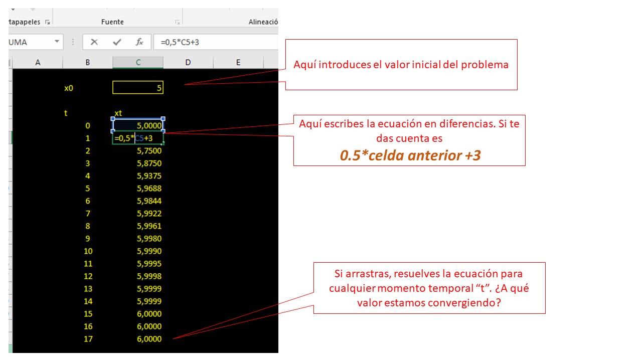
FIG1. Example of how to write it in Excel

On this screen, what we have done is write this equation \[ x_{t+1}=0.5x_{t}+3 \] and solve it using Excel.

Next, let’s write in Excel the solution we obtained:

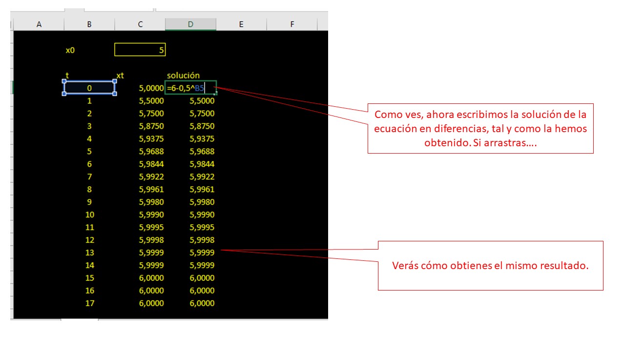
FIG2. Example of how to write it in Excel

\[ x_{t}=6-0.5^{t} \]

it should give the same result.

What is the advantage of using this equation $x_{t}=6-0.5^{t}$ versus using $x_{t+1}=0.5x_{t}+3$? If you realize, in Excel it takes you the same time. But if you have to do a calculation by hand, and I ask you how much do you make $x$ at $t=100$?. If you use the equation of the solution, you have it in a second: \[ x_{100}=6-0.5^{100} \]

However, with the initial equation, you will have

\[ x_{100}=0.5x_{99}+3 \]

And you need to know how much $x_{99}$ makes. But $x_{99}$ depends on $x_{98}$, and… so on.

CLASS 2: Convergence to equilibrium: qualitative analysis

One of the interests of studying these equations is to try to do predictions that, in this case, make some economic sense. What types of predictions do interest us?

What will happen to my variable in the next $k$ periods?

What will happen in the long term with my variable?

Will it suffer fluctuations or have a monotonous (increasing/decreasing) behavior?

Exercise

Solve, using Excel, the following difference equations and comment on which of them converge to equilibrium and which criterion they satisfy. Solve for $x_{0}=$5 and for $t=1,2,....,20$ and make the corresponding graph

\[ x_{t}=0.5x_{t-1}+3 \]

\[ x_{t}=-0.5x_{t-1}+3 \]

\[ x_{t}=1.5x_{t-1}+3 \]

\[ x_{t}=-1.5x_{t-1}+3 \]

\[ x_{t}=0.5x_{t-1} \]

\[ x_{t}=-0.5x_{t-1} \]

\[ x_{t}=1.5x_{t-1} \]

\[ x_{t}=-1.5x_{t-1} \]

sol

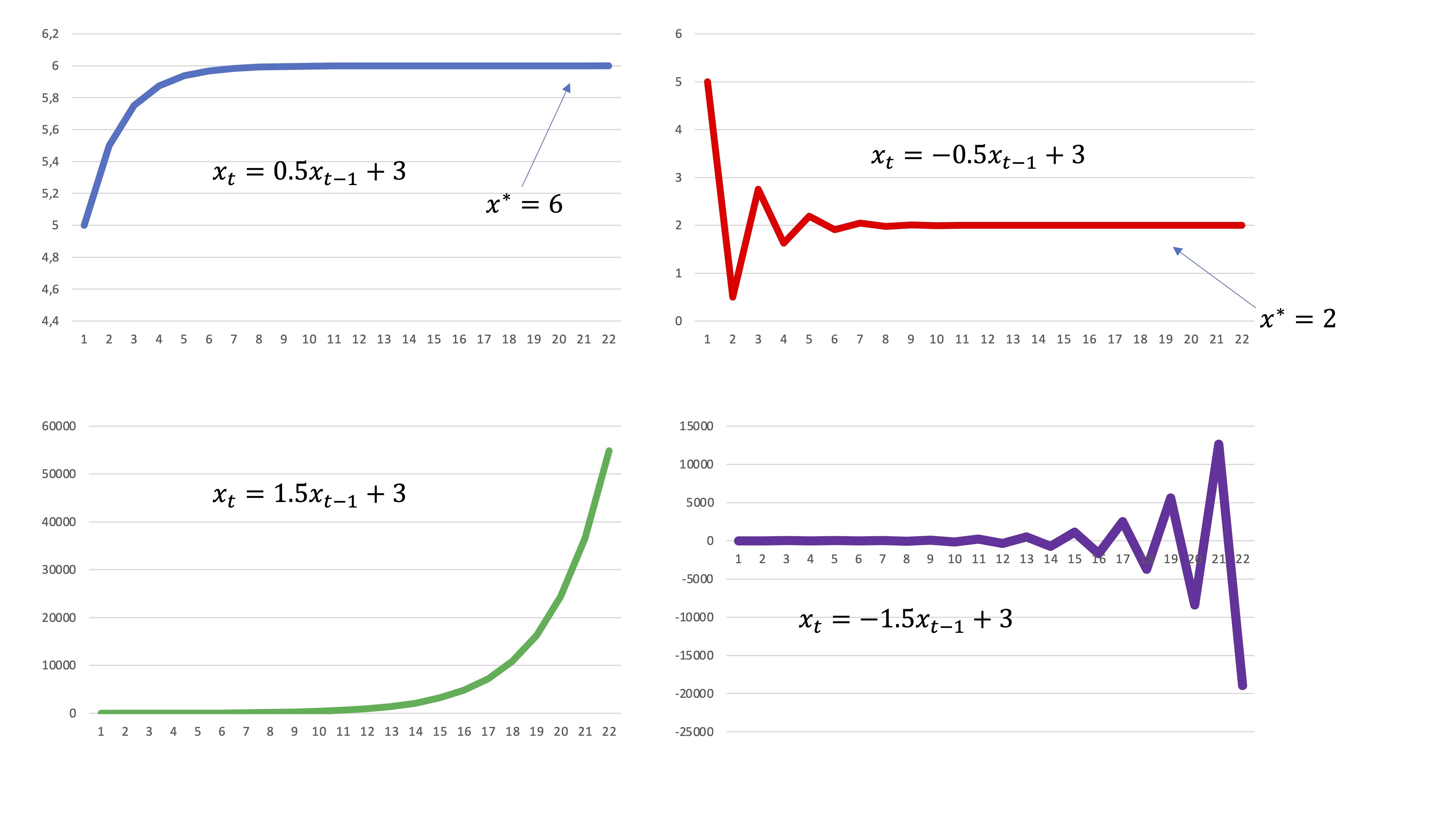
FIG1.

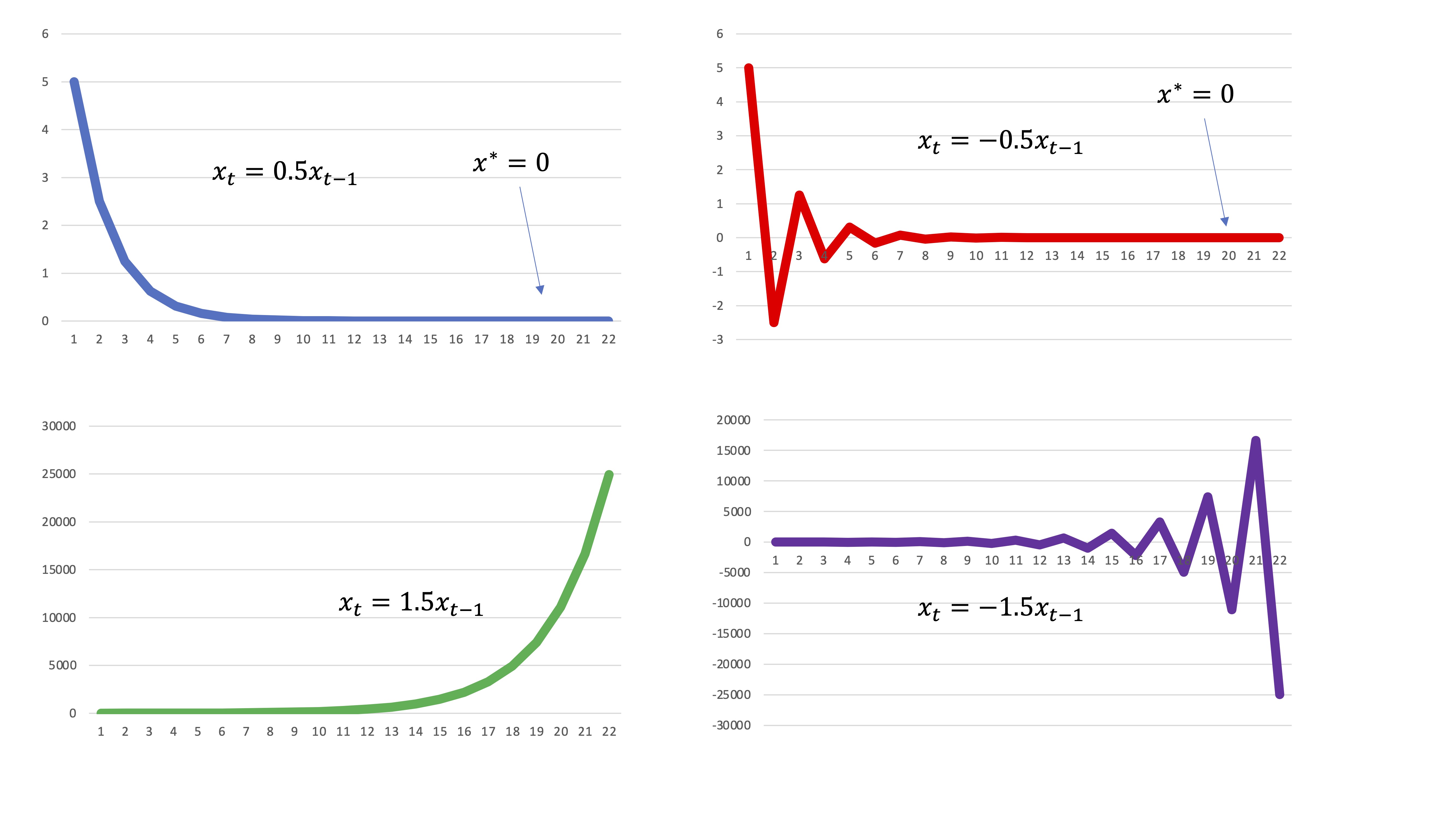
FIG2.

To the first question we will answer using the general solution of the equation (you know how to do it). However, to the other two questions, we will respond by analyzing the parameters. Doing this is called “analyzing qualitatively” the difference equation. With the charts you’ve done previously in Excel, you’ll find it easy to think about.

Case 1

\[ x_{t+1}=ax_{t} \]

Equilibrium: $x^{*}=0$

General solution: $x_{t}=a^{t}x_{0}$

if $t\rightarrow\infty$?

Then,

if $\left|a\right|<1$, is asymptotically stable (converges to equilibrium, which is zero) and if $\left|a\right|>1$, it is asymptotically unstable (diverges from equilibrium)

Case 2 \[ x_{t+1}=ax_{t}+b \]

equilibrium: $x^{*}=\frac{b}{1-a}$

General solution: $x_{t}=x^{*}+a^{t}\left(x_{0}-x^{*}\right)$

if $t\rightarrow\infty$?

Then,

if $\left|a\right|<1$, is asymptotically stable (converges to equilibrium, which is $x^{*}=\frac{b}{1-a}$) and if $\left|a\right|>1$, it is asymptotically unstable (diverges from equilibrium)

But, one thing, look at what happens if $a<0$. In any of these two formulas of the general solution

\[ \begin{cases} x_{t}=a^{t}x_{0}\\ x_{t}=x^{*}+a^{t}\left(x_{0}-x^{*}\right) \end{cases} \]

when $a$ (negative) you raise it to even power, the result will be positive while if you raise it to odd power, it will be negative (for example, $x_{1}=-0.5x_{0},x_{2}=0.25x_{0},x_{3}=-0.125x_{0}$, etc… So, if the parameter is negative, the solution of the equation we say that it presents cycles. These cycles can be convergent (to equilibrium) or divergent. You have been able to verify it with the solutions made in Excel, in FIG1 and FIG2

Class 3: Equations in second-order differences

We are going to “complicate” our model a little more. We will allow that there is now one more time delay in the difference equation. For example:

A second-order homogeneous

\[ x_{t}+a_{1}x_{t-1}+a_{2}x_{t-2}=0, \]

remember that it can also be written like this: \[ x_{t+2}+a_{1}x_{t+1}+a_{2}x_{t}=0. \]

A non-homogeneous:

\[ x_{t}+a_{1}x_{t-1}+a_{2}x_{t-2}=b, \]

\[ x_{t+2}+a_{1}x_{t+1}+a_{2}x_{t}=b \]

A non-homogeneous whose independent term is a function of $t$ (called non-autonomous)

\[ x_{t}+a_{1}x_{t-1}+a_{2}x_{t-2}=b^{t+2}, \] or also \[ x_{t+2}+a_{1}x_{t+1}+a_{2}x_{t}=b^{t} \]

As you can see, we have homogeneous and non-homogeneous again. In the case of the non-homogeneous, we can have independent terms that are constants (what we call an autonomous equation) while we can have independent terms that are a function of $t$ (in the table you have an example of the many that could be put). Doesn’t want to say that in the first-order case you can’t have equations no autonomous, simply, if you know how to solve them in the case of second order, you will have no problem solving the first order.

Homogeneous solution

The solution of the homogeneous equation is to obtain the polynomial characteristic. As we have seen before, the solutions of these equations they look like $x_{t}=r^{t}x_{0}$. If we substitute conveniently,

\[ x_{t+2}+a_{1}x_{t+1}+a_{2}x_{t}=0\Rightarrow r^{t}x_{0}+a_{1}r^{t+1}x_{0}+a_{2}r^{t+2}x_{0}=0 \]

So, for this to be a solution, taking out common factor: \[ r^{t}(r^{2}+a_{1}r+a_{2})=0 \]

From here, we get what we know as the characteristic equation, if $r\neq0$:

\[ (r^{2}+a_{1}r+a_{2})=0 \]

From this equation, we get its roots (in this course, we will only work with real roots).

Case 1: distinct real roots

The solution of the homogeneous shall be of the type

\[ x_{t}=A(r_{1})^{t}+B(r_{2})^{t} \]

where $r_1.r_2$ are the roots of the characteristic equation. You must look for the value of $A$,$B$ using-for-this- information of $x_0$ and $x_1$.

Case 2: Double Real Roots

In this case, the solution of the homogeneous, will be

\[ x_{t}=(A+Bt)r^{t} \]

where $r$ is the double root of the characteristic equation. You must look for the value of $A$,$B$ using-for-this- information of $x_0$ and $x_1$.

Stability of equations in differences of order 2

The equation in differences will converge to equilibrium (if it has one) or will be stable if and only if:

Then,

The roots of the characteristic equation are BOTH in absolute value less than one. In any other case, we will say that the equation is unstable

Case 3: General solution=homogeneous solution + particular solution

There is a very useful result in the case of linear difference equations (the ones we study this course). The general solution equals the sum of the solution of the corresponding homogeneous equation plus a particular solution. I mean:

\[ x_{t}=x_{t}^{h}+x_{t}^{p} \]

A particular solution is a function (or constant) that solves $x_{t}$ under some circumstances. Let’s see some examples

In the case of the autonomous equation, we have a clear value that solves, in particular, the equation: the equilibrium. In this case, the equilibrium will be the value of $x^{*}$ such that

\[ x^{*}+a_{1}x^{*}+a_{2}x^{*}=b\Rightarrow x^{*}=\frac{b}{(1+a_{1}+a_{2})} \]

For this equilibrium to exist, note that $a_{1}+a_{2}\neq-1$.

This, then, is a particular solution. If we want to solve the difference equation, we only have to solve the homogeneous and, then add the equilibrium

Example: Solve \[ x_{t}=5x_{t-1}-6x_{t-2}+10 \]

The homogeneous consists of: $x_{t}-5x_{t-1}+6x_{t-2}=0$

The characteristic equation $r^{2}-5r+6=0$ where $r_{1}=3.r_{2}=2$

The solution of the homogeneous is, then $x_{t}^{h}=A3^{t}+B2^{t}$

On the other hand, we have to calculate a particular one. As it is autonomous and balanced, this equilibrium is a particular solution:

$x^{*}==$5

The general solution will be: \[ x_{t}=A3^{t}+B2^{t}+5 \]

QUESTION: Is it stable?

ANSWER: No, the roots of the characteristic equation are, in value absolute, greater than one.

It is possible to obtain the value of $A$ and $B$ if they provide us with the value from $x_{0}$y $x_{1}.$ What will be the general solution if $x_{0}=10.x_{1}=12$?

\[ x_{0}=A3^{0}+B2^{0}+5=10\Rightarrow A+B=5 \]

\[ x_{1}=A3^{1}+B2^{1}+5=12\Rightarrow3A+2B=7 \]

If you solve the system, you will get: \[ x_{t}=-3\times3^{t}+8\times2^{t}+5 \]

as a general solution.

Autonomous equation without equilibrium

In this other case:

\[ x_{t}+2x_{t-1}-3x_{t-2}=16 \]

Note that $a_{1}+a_{2}=-1$, so we don’t have an equilibrium. In that In this case, we must find another way to solve it. Let’s propose a Particular solution that looks like this:

\[ x_{t}=Ct, \] it makes sense. Having no equilibrium, we expect the trajectory to have an increasing trend. In such a way that we will have to look for how much $C$ makes. To do this, note that $x_{t-1}=C(t-1)$ and that $x_{t-2}=C(t-2)$. Now, replacing in the equation:

\[ Ct+2C(t-1)-3C(t-2)=16 \]

Where we get that \[ 4C=16\Rightarrow C=4 \]

so \[ x_{t}=4t \]

it is, then, a particular solution. If we want to solve the difference equation, we only have to solve the homogeneous one, and then add the particular:

The homogeneous consists of: $x_{t}+2x_{t-1}-3x_{t-2}=0$

The characteristic equation $r^{2}+2r-3=0$ where $r_{1}=-3.r_{2}=1$

The solution of the homogeneous is, then $x_{t}^{h}=A(-3)^{t}+B$

On the other hand, we already have the particular one. So, the general solution will be

\[ x_{t}=A(-3)^{t}+B+4t \]

Is it stable?

ANSWER: No, the roots of the characteristic equation are, in value absolute, greater (or equal) than one.

In the case of the non-autonomous equation, the independent term will depend of $t$ For example:

\[ x_{t}-5x_{t-1}+6x_{t-2}=4^{t}+3 \]

Now, a particular solution cannot be the equilibrium, since this equation does not have (see that $4^{t}$ is not a constant value and an equilibrium must be). If you notice, $x_{t}-5x_{t-1}+6x_{t-2}=4^{t}+3$ is telling us that, operating with the $x$, we must reach this solution $4^{t}+3$. What is It makes us assume that the particular solution is like this: $x_{t}^{p}=C4^{t}+D$ and we look for the values of $C$ and $D$ so that the equation is satisfied and that, therefore, it is a particular solution. In this case,

\[ x_{t}=C4^{t}+D \]

\[ x_{t-1}=C4^{t-1}+D \]

\[ x_{t-2}=C4^{t-2}+D \]

Substituting in our equation,

\[ C4^{t}+D-5(C4^{t-1}+D)+6(C4^{t-2}+D)=4^{t}+3 \]

taking out common factor: \[ C4^{t}(-5\times 4^{-1}+6\times4^{-2})+D-5D+6D=4^{t}+3 \]

I mean

\[ C4^{t}\times\frac{-7}{8}+2D=4^{t}+3 \]

In order for this equality to be satisfied, \[ C=\frac{-8}{7},D=\frac{3}{2} \]

We already have the particular solution! \[ x_{t}=\frac{-8}{7}4^{t}+\frac{3}{2} \]

If we want to solve the difference equation we only have to solve the homogeneous one and, then, add the particular one:

Example: Solve

\[ x_{t}=5x_{t-1}-6x_{t-2} \]

The homogeneous consists of: $x_{t+2}-5x_{t+1}+6x_{t}{\color{red}=0}$

The characteristic equation $r^{2}-5r+6=0$ where $r_{1}=3.r_{2}=2$

The solution of the homogeneous is, then $x_{t}^{h}=A3^{t}+B2^{t}$

On the other hand, we have to calculate a particular one. The above solution is a particular one

$x_{t}=\frac{-8}{7}4^{t}+\frac{3}{2}$

The general solution will be: \[ x_{t}=A3^{t}+B2^{t}+\frac{-8}{7}4^{t}+\frac{3}{2} \]

It is possible to obtain the value of $A$ and $B$ if they provide us with the value from $x_{0}$ and $x_{1}.$ What will be the general solution if $x_{0}=10.x_{1}=12$?

In short

In short, if your equation is of this type:

\[ x_{t}+a_{1}x_{t-1}+a_{2}x_{t-2}=b^{t} \]

Try $x_{t}=Cb^{t}$

If it is of this type

\[ x_{t}+a_{1}x_{t-1}+a_{2}x_{t-2}=b_{1}^{t}+b_{2}, \]

test with $x_{t}=Cb^{t}+D$

If it is a polynomial:

\[ x_{t}+a_{1}x_{t-1}+a_{2}x_{t-2}=b_{1}t^{2}+b_{2} \]

test with $x_{t}=Cb_{1}t^{2}+Db_{1}t+E$ (with polynomials it is advisable enter all powers even if they do not appear explicitly).

NOTE: If one of the roots matches $b$, then you should try with $x_{t}=C\times t\times b^{t}$.

Class 4: Differential Equations (I)

We have already seen in part 1 of this topic that we could consider time as a discrete variable, that is, a sequence of Natural numbers \[ t=\{0,1,2,3,4,5....\} \]

or a continuous variable, such that \[ t\in [0.10] \]

that indicates any moment in time from time $t=0$ up to $t=10$ (for example, $t=1,387)$, something that -when time is considered as a discrete variable- cannot occur.

First-order differential equations

If a function, $x$, depends on time (i.e. $x(t)$), where that function you can think of as the stock price that, at each moment $t$, provides us with a market value, we can analyze how it changes in the face of “marginal” increments of the time variable. That is, we will use the derivative:

\[ \frac{\mathrm{d}x}{\mathrm{d}t} \]

The derivative tells us: "the increase of the variable $x$ if time increases a very small quantity. By the way, as $x$ in our models only depends on time, you can write the derivative as $x'$. Note that there is also a notation widely used to talk about the derivative of a time-dependent function:

\[ \dot{x} \]

yes, with a little dot.

Well, remember that our goal is going to solve a linear differential equation as follows

\[\begin{equation} x'=ax+b\label{eq:EDO} \end{equation}\]

so that, we get a solution, which is the function $x(t):$

Solving a differential equation implies finding a function of time that gives, to each value of $t$, a value for $x$.

On the other hand, do not forget that a first result that we already calculated in the equations in differences was the equilibrium. Equilibrium is again, in this case, the idea of a value of $x$ for which the derivative is zero, that is, for which the function is constant

Summary:

We call equilibrium $x^{*}$ from a differential equation a constant value that satisfies the equation. To get it, we make $x'=0$ in the equation \[ x'=ax+b, \] then \[ 0=ax^{*}+b \]

where

\[ x^{*}=\frac{-b}{a} \]

is the equilibrium.

Note that, an existence condition for the equilibrium is $a\neq0$.

So, equilibrium is a constant value, of reference, to which the variable will tend in the long term if the model is stable. If it is not stable, the variable will pass through equilibrium but it will never stay in it.

Remember

Balance	Differential Equation	Equation in differences
$x^*=$	$\frac{-b}{a}$	$\frac{b}{1-a}$

Solving differential equations of order 1.

Let’s see how to solve the first order differential equations of the type \[ x'=ax+b \]

in its different versions of interest.

Case 1: $a\neq0$,$b=0$

In this case, we have a first-order linear differential equation and homogeneous (remember, because $b=0).$ Let’s solve it using: THE FUNDAMENTAL THEOREM OF CALCULUS!

\[ \frac{\mathrm{d}x}{\mathrm{d}t}=ax \]

As you can see, I use the notation with $\mathrm{d}x,\mathrm{d}t$, because it’s going to be more comfortable for me. To begin with, I leave everything aside that has to do with the $x$ and, in the other, what it has to do with with the $t$, then: \[ \frac{\mathrm{d}x}{x}=a\mathrm{d}t \]

Now, to get rid of the “differentials,” since I want a solution for $x$, I use the Fundamental Theorem of Calculus that says:

\[ \int\frac{\mathrm{d}x}{x}=a\mathrm{\int d}t \]

from what I get:

\[ \ln(x)=at+C \]

(remember to put the integration constant). Since I want a solution for the $x$, I must undo the logarithm. I use the exponential:

\[\begin{equation} e^{\ln(x)}=e^{at+C} \end{equation}\]

from where,

\[ x=e^{at}e^{C} \]

I already have the solution:

\[\begin{equation} x(t)=e^{at}A,\label{eq:homog_orden1} \end{equation}\]

where $A$ is any constant. If I know the initial value, for example, I know that $x(0)=x_{0}$, I can use it to compute $A$:

\[ x(0)=e^{a\times0}A=x_{0}\Rightarrow A=x_{0}, \]

from what we have

\[ x(t)=e^{at}x_{0}, \] which is the solution we were looking for.

case 2 $a\neq0$,$b\neq0$

This equation is not homogeneous: we say it is autonomous when $b\neq0:$

\[ \frac{\mathrm{d}x}{\mathrm{d}t}=ax+b \]

To solve this equation, let’s first define its equilibrium. \[ x^{*}=\frac{-b}{a}, \]

that we already know that equilibrium is a value of $x$ that satisfies the equation. Now, let’s use the well-known principle that the general solution of the equation will be the sum of the solution of the homogeneous and the particular. The homogeneous has been solved before, I mean: \[ x^{h}(t)=e^{at}A. \]

The general solution will be the sum of both, therefore \[ x(t)=e^{at}A-\frac{b}{a} \]

Now, if we have to $x(0)=x_{0}$, then,

\[ x(0)=e^{a\times0}A-\frac{b}{a}=x_{0}\Rightarrow A=x_{0}+\frac{b}{a} \]

Plugging in the obtained value

\[ x(t)=e^{at}\left[x_{0}+\frac{b}{a}\right]-\frac{b}{a}, \] we rewrite the solution as \[ x(t)=x^{*}+e^{at}\left[x_{0}-x^{*}\right]. \]

If you notice, it looks like the analog solution in differences!

Look

	Differential Equation	Equation in differences
Equation	$x'=ax$	$x_{t}=ax_{t-1}$
	Solution $x(t)=e^{at}x_{0}.$	$x(t)=e^{at}x_{0}$
Equation	$x'=ax+b$	$x_{t}=ax_{t-1}+b$
	Solution $x(t)=x^{}+e^{at}\left[x_{0}-x^{}\right]$	$x_{t}=x^{}+a^{t}\left[x_{0}-x^{}\right]$

Convergence to equilibrium: qualitative analysis

In the same way that we studied the long-term trend in in the case of equations in differences, we do the same with the differential equations. However, there is good news: They are easier! And why is that? As you already know, analyzing in the long term consists of to see what happens to the equation if $t\rightarrow\infty$. In the solution case, $x(t)=x^{*}+e^{at}\left[x_{0}-x^{*}\right]$, such as we have an exponential, there are only two possibilities: if $a>0$, then $\lim_{t\rightarrow\infty}e^{at}=\infty$ and, if $a<0$, then $\lim_{t\rightarrow\infty}e^{-at}=0$. In this way, if the parameter is positive, we know that we will not converge to equilibrium whereas, if the parameter is negative, yes.

Class 5: Second-order differential equations

We are going to “complicate” our model a little more. We will allow that the second derivative now appears in the differential equation, having second-order linear differential equations Homogeneous equation

\[ x''+a_{1}x'+a_{2}x=0 \]

Non-homogeneous (autonomous) equation

\[ x''+a_{1}x'+a_{2}=b \]

Non-homogeneous (non-autonomous) equation

\[ x''+a_{1}x'+a_{2}x=be^{t} \]

Homogeneous solution

The solution of the homogeneous equation needs to obtain the characteristic equation. As we have seen before, the solutions of these equations (first order) they are like $x(t)=e^{rt}x_{0}$. If we resemble the idea and substitute conveniently

\[ x''+a_{1}x'+a_{2}x=0\Rightarrow r^{2}e^{rt}x_{0}+a_{1}re^{rt}x_{0}+a_{2}e^{rt}x_{0}=0 \]

So, for this to be a solution: \[ e^{rt}x_{0}(r^{2}+a_{1}r+a_{2})=0 \]

From here, we get what we know as the characteristic equation, since it has to be solved, if $r\neq0$

\[ (r^{2}+a_{1}r+a_{2})=0 \]

From this equation, we get its roots (in this course, we will only work with real roots).

Distinct real roots

The solution of the homogeneous shall be of the type

\[ x(t)=Ae^{r_{1}t}+Be^{r_{2}t} \]

Double real roots

In this case, the solution of the homogeneous, will be

\[ x(t)=(A+Bt)e^{rt} \]

General solution=homogeneous solution + particular solution

We need this result again to be able to solve equations NOT homogeneous.

\[ x_{t}=x_{t}^{h}+x_{t}^{p}, \]

let’s look at the different cases.

Case 1: autonomous

\[ x''+a_{1}x'+a_{2}=b \]

To get the equilibrium, we do $x''=x'=0$

With Equilibrium

In the case of the autonomous equation, we have a clear point that solves, in particular, the equation: the equilibrium. In this case, the equilibrium will be the value of $x^{*}$ such that

\[ a_{2}x^{*}={\color{red}b}\Rightarrow x^{*}=\frac{b}{a_{2}} \]

For this balance to exist, note that $a_{2}\neq0$.

This, then, is a particular solution. If we want to solve the differential equation, we only have to solve the homogeneous and, then add the equilibrium.

Example: Solve

\[ x''=5x'-6x+10 \]

The homogeneous consists of: $x''-5x'+6x=0}$

The characteristic equation $r^{2}-5r+6=0$ where $r_{1}=3.r_{2}=2$

The solution of the homogeneous is, then $x_{t}^{h}=Ae^{3t}+Be^{2t}$

On the other hand, we have to calculate a particular one. As it is autonomous, equilibrium—if it exists—is a particular solution:

$x^{*}=\frac{10}{6}=\frac{5}{3}$

The general solution will be: \[ x(t)=Ae^{3t}+Be^{2t}+\frac{5}{3} \]

It is possible to obtain the value of $A$ and $B$ if they provide us with the value of $x(0)$ and $x'(0).$ What will be the general solution if $x(0)=\frac{5}{3},x'(0)=1$?

Then \[ x(0)=A+B+\frac{5}{3}=\frac{5}{3}\Rightarrow A+B=0 \]

on the other hand, we need to make the derivative of $x(t):$

\[ x'=3Ae^{3t}+2Be^{2t} \]

Now we evaluate it at 0,

\[ x'(0)=3A+2B=1 \]

If you solve the system, you will get: \[ x(t)=e^{3t}-e^{2t}+\frac{5}{3} \]

as a general solution.

Case 2: Non-autonomous equation

In the case of the non-autonomous equation, the independent term will depend of $t.$ For example:

\[ x''=5x'-6x+e^{-2t}+10 \]

Now, a particular solution cannot be the equilibrium, since that this equation does not have one (see that $e^{-2t}$ is not a constant value and an equilibrium must be). We use, again, the method indetermined coefficients. This method works in very simple cases (such as the ones we will address here) and is based on trying to figure out what it looks like has the solution of the differential equation. If you notice, $x''-5x'+6x=e^{-2t}$, is telling us that, operating with the $x$, we must arrive at this solution $e^{-2t}$. What is done it is assumed that the particular solution is like this: $x_{t}^{p}=Ce^{-2t}$ and we look for the value of $C$ so that the equation is satisfied and that, therefore, it is a particular solution. In this case,

\[ x^{'p}=Ce^{-2t} \]

from where ${x}^{'p}=-2Ce^{-2t}$ and where ${x}^{''p}=4Ce^{-2t}.$ So, replacing:

\[ 4Ce^{-2t}+10Ce^{-2t}+6Ce^{-2t}=e^{-2t} \]

\[ 20Ce^{-2t}=e^{-2t}\Rightarrow C=\frac{1}{20}. \]

If we want to solve the complete equation, we just have to solve the homogeneous one and, then, add the particular one:

As we already have the homogeneous of the previous case

\[ x(t)=Ae^{3t}+Be^{2t}+\frac{1}{20}e^{-2t} \]

Ideas:What functions to use for the particular in non-autonomous?

In short, if your equation is of this style:

\[ x''+a_{1}x'+a_{2}x=be^{t} \]

Test $x(t)=Cbe^{t}$

IF it is of this style

\[ x''+a_{1}x'+a_{2}x=b_{1}e^{t}+b_{2}, \]

test with $x(t)=Cb_{1}e^{t}+D$

If it is a polynomial:

\[ x''+a_{1}x'+a_{2}x=b_{1}t^{2}+b_{2} \]

test with $x(t)=Cb_{1}t^{2}+Db_{1}t+E$ (with polynomials it is advisable enter all powers even if they do not appear explicitly).

NOTE: If one of the roots matches $b$, then you should try with $x(t)=C\mathbf{t}e^{t}$.

Solved Exercises to Practice

The price of a good follows the following differential equation

\[ P'=-6P+270 \]

Get the price equation for all $t$ and say where it converges in the long run.

solution

Being a linear Differential Equation (first order) its equilibrium is $P^{*}=\frac{270}{6}=45$ and its solution: \[ P(t)=45+e^{-6t}\left(P_{0}-45\right) \]

as we see, $\lim_{t\rightarrow\infty}P=45$ , since the term $e^{-6t}\rightarrow0$ when $t\rightarrow\infty.$

It is known that the number of football fans varies depending on the fans that there are in every moment of time, since the fans current recruit new fans among their friends, so that which varies the number of fans at any given time (measured in hours) is equal to 0.1% of the number of fans there are at every moment. Knowing that there are currently 20 million followers of Spanish football, how many hours will have to pass for it to triple the number of followers? What if the number of followers was 30 Million?

solution

Let $A$ be the number of fans, and let $A(t)$ be the function it describes the fans there are in a moment $t$ of time. In the text fans are said to evolve as follows:

\[ \frac{\mathrm{d}A}{\mathrm{d}t}=0.001A \]

The solution to this equation is \[\begin{equation} A(t)=e^{0.001t}A_{0} \end{equation}\]

In this case, including the initial condition: \[\begin{equation} A(t)=e^{0.001t}20 \end{equation}\]

To know when they will triple ($A(t)=60)$ we must clear $t$:

\[ 60=e^{0.001t}20\Rightarrow3=e^{0.001t}\Rightarrow1.098=0.001t\rightarrow t=1098 \]

Let be the demand and supply functions of an adjustment model of dynamic pricing: $Q_{d}=4-2P(t)+5\frac{dP}{dt},Q_{s}=-6+3P(t)$. Likewise, it is known that the variation of the price at each moment t is equal to 60%of excess demand (Walrasian hypothesis). Get:

The price time path for the initial conditions $P(0) = $8.

What is the price trend for a sufficient period of time long?? Can it be said that the model is dynamically stable? Justify the answer.

solution

As specified in the model \[ P'=0.60(D-S) \]

I mean

\[ P'=0.60(4-2P+5P'+6-3P), \]

then

\[ P'=6-3P+3P' \] and, therefore, \[ -2P'=6-3P\Rightarrow P'=-3+\frac{3}{2}P \]

The time trajectory of the price will be the solution to the first-order differential equation presented, i.e.

\[ P(t)=2+e^{\frac{3}{2}t}\left(P_{0}-2\right) \]

The intertemporal equilibrium price is the one obtained by making $0=-3+\frac{3}{2}P\Rightarrow P=2$. The perfect market is to match supply and demand with $P'=0$, which also comes out 2.

However, in the long term, this market is not dynamically stable, since for $t\rightarrow\infty$, then $P(t)\rightarrow\infty$.

t	Equation
0	\(x_{0}\)
1	\(x_{1}=x_{0}+10\)
2	\(x_{2}=x_{1}+10\)	\(x_{2}=x_{0}+10+10\)
…	…	…
T		\(x_{T}=x_{T-1}+10\)

	\(x_{t+1}=\)	\(ax_{t}\)	\(+b\)
\(\color{red}-\)	\(x^{*}=\)	\(ax^{*}\)	\(+b\)

	\(x_{t+1}-x^{*}=\)	\(a\left(x_{t}-x^{*}\right)\)	\(+0\)

	Differential Equation	Equation in differences
Equation	\(x'=ax\)	\(x_{t}=ax_{t-1}\)
	Solution \(x(t)=e^{at}x_{0}.\)	\(x(t)=e^{at}x_{0}\)
Equation	\(x'=ax+b\)	\(x_{t}=ax_{t-1}+b\)
	Solution \(x(t)=x^{}+e^{at}\left[x_{0}-x^{}\right]\)	\(x_{t}=x^{}+a^{t}\left[x_{0}-x^{}\right]\)