BLOCK 4: Advanced Optimization

• In this block, we will delve into the approach and resolution of relevant optimization problems in Economics.
• We will prepare to discuss, given the problem, if it has a solution and what kind to expect
• In addition, we will insist on graphic resolution as a way to obtain powerful ideas of the problem without making much analytical effort.

References of interest

• Stewart, J. (2009). Calculus: Concepts and contexts. Cengage Learning.
• STEWART, James; CLEGG, Daniel K.; WATSON, Saleem. Calculus: early transcendentals. Cengage Learning, 2020.
• SYDSAETER, Knut; HAMMOND, Peter. Mathematics for economic analysis. Pearson Education, 1996.
• SIMON, Carl P., et al. Mathematics for economists. New York: Norton, 1994.
• SMITH, Robert T.; MINTON, Roland B.; RAFHI, Ziad AT. Calculation of several variables: early transcendents. McGraw-Hill Interamericana, 2019.

Class 1: Review of Important Calculus Ideas

As you already know about Maths I, we are working with functions in two variables. Remember that \(f:\:\mathbb{R}^{2}\rightarrow\mathbb{R}\) is a function whose domain is contained in the set of two-dimensional reals (\(\mathbb{R}^{2})\) and the image are the real ones (\(\mathbb{R})\), from such a way that its graph is three-dimensional. For example, the \[ f(x,y)=2x+y-3, \]

represents a drawing in \(\mathbb{R}^{3}:\)

FIG1 This represents the function \(f(x,y)=2x+y-3\).

Proposed Exercise

Represent in geogebra the following functions in 3D

1. \(f(x,y)=e^{2x-y}\)

2. \(f(x,y)=(x-1)^{2}+(y+2)^{2}\)

3. \(f(x,y)=4(x+1)^{2}+(y+1)^{2}\)

4. \(f(x,y)=xy\)

Generally, it is difficult to draw functions in 3D unless we have by hand Geogebra. Remember that a way to study the most important characteristics of a 3D function is by its contour lines. To do this, the what we have is to set values of the image (in such a way that we we get rid of a variable) and clear a variable (of the two that remain) depending on the other. For example, from the function

\[ z=2x+y-3, \]

we set values of \(z\), as for example \(z=\{-1.0.2\}\)

\[ -1=2x+y-3,\:\:\:0=2x+y-3,\:\:\:2=2x+y-3 \]

and we clear the \(y\) based on the \(x\), getting:

\[ y=2-2x,\:\:\:y=3-2x,\:\:\:y=5-2x \]

as you can see, they correspond to parallel lines with negative slopes

FIG2 Some contour lines of the function, with the arrow indicating where it grows

Caution, review!

In class 5 of BLOCK 1 you can review the idea of contour lines and watch an explanatory video.

Solved Exercis

Outline the contour lines of the following functions, explaining which 2D objects (functions, conical, etc…) represent:

1. \(f(x,y)=(x-1)^{2}+(y+2)^{2}\)\(\rightarrow\) Centered circumference at point \((1,-2)\)

2. \(f(x,y)=4(x+1)^{2}+(y+1)^{2}\)\(\rightarrow\) Ellipse centered on the point \((-1,-1)\)

3. \(f(x,y)=xy\)\(\rightarrow\) Hyperbola

4. \(f(x,y)=e^{2x-y}\)\(\rightarrow\) They are straight with positive slope

On the other hand, we must remember the fundamental properties of the gradient of a function. To do this, we will show them with clear examples. Let be the function in two variables \(f\::\:\mathbb{R}^{2}\rightarrow\mathbb{R}\), we will define the gradient as the vector \(\nabla f\) that has by components the partial derivatives of the function \(f\), i.e.

\[ \nabla f(x,y)=\left[\frac{\partial f}{\partial x},\frac{\partial f}{\partial y}\right]. \]

The gradient, just remember, is key to solving optimization problems. Among its properties, are

• It is perpendicular to each contour line at each point (FIG4)

• marks the direction with two senses: the steepest ascent and descent. (FIG5)

That is, if you move in the direction of the gradient (\(\nabla f(x,y))\) you know that you are going to reach higher levels of function as soon as possible. If you choose the sense negative (\(-\nabla f(x,y)\)) you will move as soon as possible towards values smaller than the function. This clearly has a relationship to maximizing/minimizing a function \(f(x,y)\)

FIG4 gradient properties (1)

FIG5 gradient properties (2)

You will understand, then, that the gradient of a function will have to be present in the resolution of optimization problems. Review block 3, where you have the optimization theory that you should know so far.

Caution, review!

In class the optimization problem will be solved with equality restrictions of the Mathematics I exam.

Class 2: Posing optimization problems with inequality constraints

In general, we will be interested in raising problems where, before a set of possible options, let’s be able to see what is the best and the worst. That’s called: optimize. In mathematics, we will pose optimization problems such as the one that is represents in this problem 1:

Problem 1

\[\begin{equation} \mathrm{opt}f(x,y) \end{equation}\]

subject to \[ (x,y)\in X \]

Where \(f(x,y)\) is the objective function (which we want to optimize) and \(X\) is known as the feasible set: that is, it is the place where we look for the values of \((x,y)\) to be able to solve our optimization problem. In this course, we will assume that \(X\subseteq\mathbb{R}^{2}\), that is, the feasible options will be pairs of real numbers in two dimensions and that, in addition, these will be a subconjutno of said space. In FIG 1, we show the 3D graphic of an objective function represented on a set of feasible solutions \(X\) formed by a square.

FIG1 We represent the function \(f(x,y)=\ln(1+x^{2}+y^{2})-x^{2}\), with \(X=\left\{ (x,y)\in\mathbb{R}^{2}:-3\leq x\leq3,-1\leq y\leq4\right\}\)

On the other hand, if our goal is to maximize or minimize, we will reformulate the problem 1: we will have to write \(\max/\min\) according to what corresponds.

Remember that our goal will be to look for global optimums: that is, the best/worst of all candidates for highs and lows of the objective function. In FIG2, we represent the overall maximum and minimum of the function \(f(x,y)=\ln(1+x^{2}+y^{2})-x^{2}\), for the values \((x,y)\in X\), as well as the local maximums and minimums. Remember that general methods of searching for optimums usually find local critical points that, later, we will have to analyze to know which of them are global.

FIG2 We represent the function \(f(x,y)=\ln(1+x^{2}+y^{2})-x^{2}\), with \(X=\left\{ (x,y)\in\mathbb{R}^{2}:-3\leq x\leq3,-1\leq y\leq4\right\}\)

In general, in this chapter we will work with sets feasible \(X\) conformed by inequalities as we propose in the problem 2

Problem 2

\[\begin{equation} \mathrm{opt}f(x,y) \end{equation}\]

subject to \[\begin{equation} \begin{cases} g_{1}(x,y)\leq k_{1}\\ ...\\ g_{m}(x,y)\leq k_{m} \end{cases}\label{eq:rest} \end{equation}\]

Where, as a novelty, the functions \(g_{i}(x,y)\), for \(i=1,... m\) are the inequality constraints that make up the set of solutions Feasible. We will use, as an agreement, inequalities of the type less than or equal.

In Economics there are many examples of interest. Here we think about a few:

-P1. Maximize the \((U)\) utility that the purchase brings to an individual of two goods \((x,y)\) subject to a budgetary constraint:

\[ \max U(x,y) \] \[ p_{x}x+p_{y}y\leq R, \] where \(p_{x},p_{y}\) are the prices of goods, \(R\) is the rent and \(U\::\mathbb{R}_{++}^{2}\rightarrow\mathbb{R}_{+}\)

• P2. Choose how much capital \((k)\) and workers \((L)\) to hire for minimize the cost if you want to produce, at least \(u\) units product:

\[ \min C(K,L) \] \[ f(k,L)\geq u, \]

where \(C\) is a cost function, such that \(C\::\mathbb{R}_{++}^{2}\rightarrow\mathbb{R}_{+}\) and \(f\) a production function \(f\::\mathbb{R}_{++}^{2}\rightarrow\mathbb{R}_{+}\).

• P3. Choose levels of advertising on social networks \((x)\) and television \((y)\) as well as the price \((p)\) that maximize the profit of a company, subject to a certain restriction (e.g. spending on both average must be less than 5 M euros) and the price must be between 2 and 5 euros:

\[ \max pV(p,x,y)-(x+y) \] \[ x+y\leq5, \] \[ 2\leq p\leq5, \]

where \(V\) are the sales of the product associated with the price and expenses in advertising, such that \(V\::\mathbb{R}_{+++}^{3}\rightarrow\mathbb{R}_{+}\)

---

Solved Exercise

It discusses whether the examples proposed above fit with the problem of optimization with inequality constraints that has been enunciated at the beginning of the class.

-P1. It fits perfectly, since it consists of a maximization problem with an inequality constraint of the type “less than or equal to” -P2.No, you would have to write \(-f(k,L)\leq-u\), to have an inequality of the type requested. - P3. Two inequalities would have to be written \(\begin{cases} -p\leq-2\\ p\leq5 \end{cases}\)

NOTE: It is important to always rewrite inequalities in this way, since all the analytical procedures that we are going to use depend on that the restrictions are written with that sense of inequality: “\(\leq\).”

---

Exercise 2

Make the approaches of the problems of the course 6-10.

Class 3: Karush-Khun-Tucker method

Optimal conditions

Having seen all the above, we are going to find an algorithm that will allow us to look for the critical points in an optimization problem with inequality restrictions.

CAUTION, review!

A critical point is that point that can be a maximum, minimum or saddle point.

The KKT method is based on the approach of a mathematical program with inequalities (remember that in this sense: \(\leq\), if you do not have to change them conveniently)

\[ \mathrm{opt}f(x,y) \]

subject to

\[ \begin{cases} g_{1}(x,y)\leq k_{1}\\ ...\\ g_{m}(x,y)\leq k_{m} \end{cases} \]

Note: in these notes we will consider that the condition of regularity that requires gradients of \(g_{i}(x,y),\:i=1,...,m\) are linearly independent.

We construct the Lagrangian function such that:

\[ \mathcal{L}(x,y,\lambda_{1},...,\lambda_{m})={ \color{red}{f(x,y)}-{\color{green}{ \lambda_{1}\left(g_{1}(x,y)-k_{1}\right)}}-...-{{\color{green}{ \lambda_{m}\left(g_{m}(x,y)-k_{m}\right)}}}} \]

so that we have in a single function the objective and the constraints. You have already done this in optimization with equality restrictions.

KKT conditions indicate that there are \(\lambda_{1},...,\lambda_{m}\in\mathbb{R}\) such that satisfy

	concept for maximum	for minimum
partial derivatives	\[ \; \; \; \; \; \; \; \; \; \; \; \; \; \; \; \; \; \; \; \; \; \; \; \; \frac{\partial\mathcal{L}}{\partial x}=0, \frac{\partial\mathcal{L}}{\partial y}=0 \]
complementary slackness	clearance \[ \begin{cases} \lambda_{1}[g_{1}(x,y)- k_{1}]=0\\ ...\\ \lambda_{m}[g_k(x,y)-k_{m}]=0 \end{cases} \]
	multipliers \(\lambda_{1},...,\lambda_{m}\geq0\)	\(\lambda_{1},...,\lambda_{m}\leq0\)
	feasibility \[ \begin{cases} g_{1}(x,y)\leq k_{1}\\ ...\\ g_{m}(x,y)\leq k_{m} \end{cases} \]

These conditions, necessary, will allow us to obtain the set of critical points \((x,y,\lambda_{1},...,\lambda_{m})\) candidates to optimal.

• The conditions of Complementary Slackness are usually choked. Pay attention to the example and use logic!
• The condition about multipliers gives us a lot of information. If we find that they are of the opposite sign, we immediately discard that critical point because it does not satisfy it.
• Feasibility implies that, once you have optimal candidates, you have to verify that they satisfy all constraints (the equations previous ones do not assure it). If not, that point is discarded.

Note: In these notes, the conditions of non-negativity (\(x,y>0\) or \(x,y\geq0\)) will not be taken into account. These will be checked on the fly, but will not be included in the Lagrangian.

---

Easy exercise Try to solve problem #5 on the course worksheet.

More complicated example

Be the optimization problem

\[ \mathrm{opt}\:f(x,y)=x^{2}+y \] subject to

\[ \frac{x^{2}}{4}+\frac{y^{2}}{9}\leq1 \]

• We write the Lagrangian:

\[ \mathcal{L}(x,y,\lambda_{1},...,\lambda_{m})=x^{2}+y-\lambda\left(\frac{x^{2}}{4}+\frac{y^{2}}{9}-1\right) \]

• We obtain the partial derivatives and equal to zero \[ \frac{\partial\mathcal{L}}{\partial x}=0\Rightarrow2x-\frac{x\lambda}{2}=0 \] \[ \frac{\partial\mathcal{L}}{\partial y}=0\Rightarrow1-\frac{2y\lambda}{9}=0 \]

• We write the conditions of complementary slackness \[ \lambda\left(\frac{x^{2}}{4}+\frac{y^{2}}{9}-1\right)=0 \]

You can actually see it as having to solve this system of equations.

\[\begin{equation} KKT\begin{cases} x\left(2-\frac{\lambda}{2}\right)=0 & (1)\\ 1-\frac{2y\lambda}{9}=0 & (2)\\ \lambda\left(\frac{x^{2}}{4}+\frac{y^{2}}{9}-1\right)=0 & (3) \end{cases} \end{equation}\]

As the system is non-linear, we advise you to systematize the search for solutions, for example, by making a tree as follows:

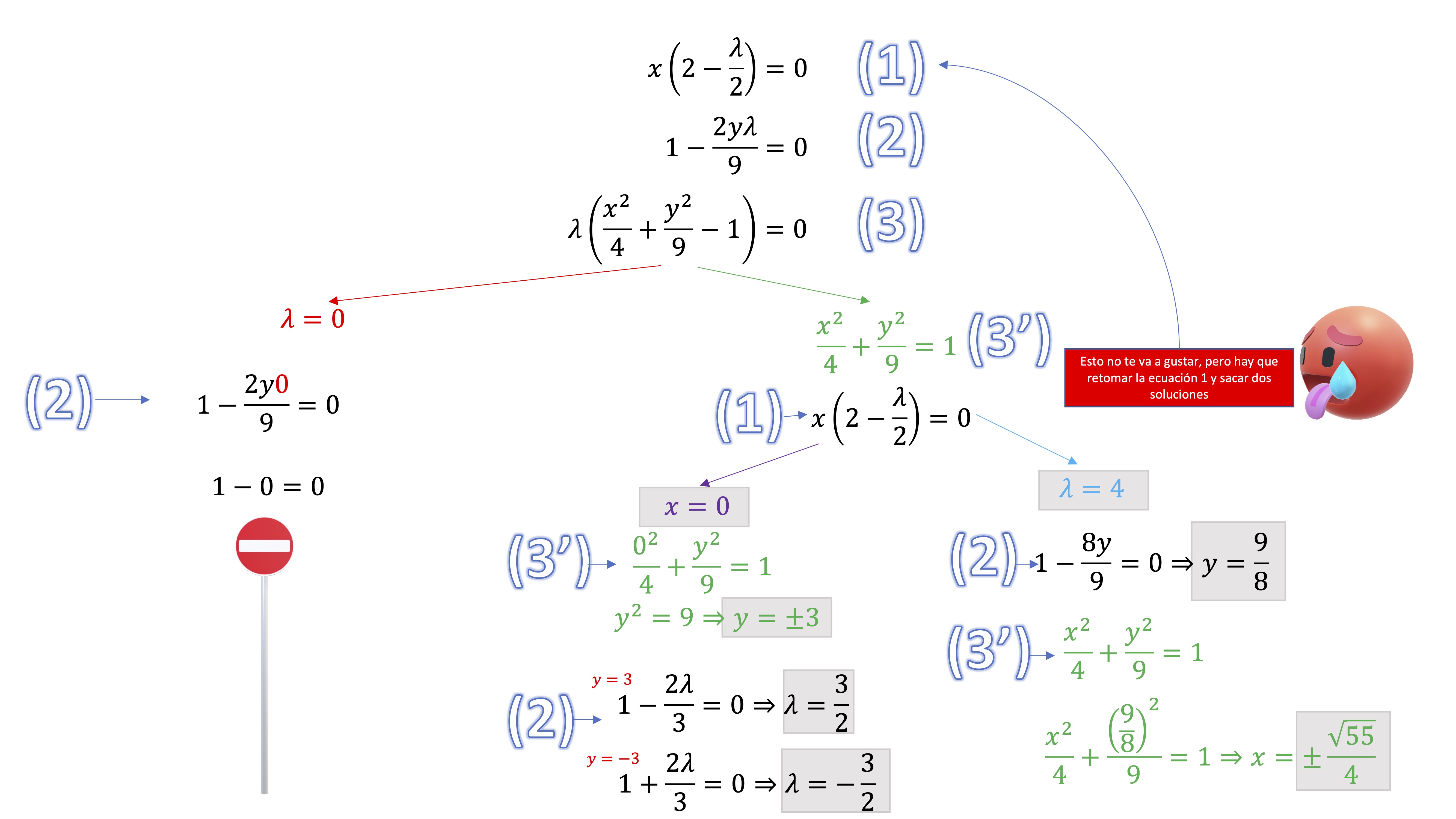
FIG1 Solution Tree

---

• Classifies the solutions obtained using the necessary conditions.

Point	1	2	3	4
\(x^*\)	0	0	\(\sqrt{55}/4\)	\(-\sqrt{55}/4\)
\(y^*\)	3	-3	\(9/8\)	\(9/8\)
\(\lambda^*\)	3/2	-3/2	\(4\)	\(4\)

Points 1,3,4 meet the Kuhn Tucker condition for maximum and point 2 with the condition for minimum.

To know more: Where do Kuhn and Tucker’s conditions come from? You don’t need to look at this, only if you’re curious.

---

Let’s understand, graphically, the particularities of the Karush-Kuhn-Tucker conditions Let’s remember, of course, briefly, the powerful idea behind the Lagrangian. Suppose we want to solve a minimization problem, such that

\[\begin{equation} \min f(x,y) \end{equation}\]

In that case, a necessary condition for the search of the minimum consisted of

\[ \frac{\partial f}{\partial x}=0,\frac{\partial f}{\partial y}=0\Rightarrow\nabla f(x,y)=(0,0) \]

That is, a minimum candidate must meet that the gradient is cancelled at that point. In FIG 2 we can intuit where this condition comes from:

FIG2 unrestricted issue

We start at any point \(A\) and going in the direction gradient negative – remember what we saw in CLASS 1 – to minimize a function, we must go in the negative direction of the gradient. We are descending as quickly as possible by the function until we reach the point where it is impossible to descend more. That point with coordinates \((x^{*},y^{*})\) is the one at which the gradient is \((0.0)\). Of course, if the gradient is different from the (0,0), that will mean that we can continue to decrease in that direction, so we must look for a point where we no longer decrease. This as far as looking for a minimum without having any restrictions is concerned.

Now, remember that if you restricted the function to a set of points, as in the following case

\[\begin{equation} \min f(x,y) \end{equation}\]

subject to

\[ g(x,y)=k, \]

you’ll be in a situation like this, where the curve red is the restriction \(g(x,y)=k\)

FIG3 point \(C\) is the best

FIG4 How did we get to the point \(C\) with what we know about calculation?

The points \(A\) and \(B\) are cut-off points of the level with restriction. Both points are feasible (they are contained in the restriction) but do not provide the lowest possible values of the target function (point \(A\) provides value 30, while that the point \(B\) provides value 40). If we move along the contour line, we will reach the point \(C\). This is a point of tangency between the contour (valued at 20) and the constraint. It’s the best, since you cannot find any other point than, satisfying the restriction, provide a lower value of the target function. Given the properties of the gradient vector that we review in class 1, we know that this will be perpendicular to the contour line at point \(C\). Also, the point \(C\) is also common for the constraint, whose gradient (\(\nabla g)\) will be perpendicular to that restriction. In this way, and as you see in the FIG 4, both the gradient of the contour line and that of the constraint they must point in the same direction (being at a point of tangency, that is, common) in such a way that they will be proportional, that is:

\[\begin{equation} \nabla f(x,y)=\lambda\nabla g(x,y) \end{equation}\]

Note that, in this case, the gradient of the function objective \(\nabla f\) and that of the restriction \(\nabla g\) are in the same address but have opposite senses (which will make \(\lambda<0)\).

Lagrange proved that this tangency condition can be achieved by the Lagrangian function \(\mathcal{L}\::\:\mathbb{R}^{3}\rightarrow\mathbb{R}\) defined how \[ \mathcal{L}(x,y,\lambda)=f(x,y)-\lambda g(x,y), \] which, subsequently, we will recover.

KKT conditions: tangency solution versus inner solution

The time has come to understand what the conditions are necessary that will allow us to look for critical points when we are in trouble with inequality constraints.

Suppose we want to solve a minimization problem, such that

\[\begin{equation} \min f(x,y) \end{equation}\]

subject to \[ g(x,y)\leq k \]

as you will assume, it will depend on the function \(f(x,y)\) and where the restriction is located, we can have two types of minimums basically:

FIG5 inner solution vs tangency solution

• inner solution

In the first case, that of the interior solution, we see that the function decreases as we approach the center of the ellipse. In this case, if you notice, the restriction allows us to optimal point that we seek consists of working as if we did not have the constraint (i.e., the optimum is at a point that satisfies \(g(x,y)<k)\). And, via the Lagrangian, we would have to

\[\begin{equation} \mathcal{L}(x,y,\lambda_{1},...,\lambda_{m})={ {\color{red}f(x,y)}-{\color{green}{ \lambda\left(g(x,y)-k\right)}}} \end{equation}\]

but, since in this case the constraint is as if it were not, we know that the necessary condition of optimal must be \(\frac{\partial f}{\partial x}=0,\frac{\partial f}{\partial y}=0\). For that to happen in the equation above, you will have to happen that \(\lambda=0\).

IDEA: if the solution is in the interior, this implies that \(\lambda=0.\) In Economics: if a resource, available in quantity limited (i.e. where a constraint operates), not used in the optimum so that it is exhausted, its limitation does not represent any role in the problem. However, until the problem is resolved, we don’t know if the solution is interior or not.

• tangency solution

In the second case, the optimal solution will be found right in the restriction \(g(x,y)=k\). Here we recover the Lagrange idea that we have reviewed before, so we will have to the gradients of the objective function and the constraint must be Proportional:

FIG6 Tangency Solution

which will imply, therefore, that when we look for solutions which are points of tangency, \(\lambda\neq0\) (in this case, as we see, when searching for a minimum, \(\lambda<0\)).

• Complementary slackness

Given the above, we must then study two possibilities of interest to search for critical points that are related to the value of the multiplier, \(\lambda=0\) (inner solution) and \(g(x,y)=k\Rightarrow\lambda\neq0\) (point of tangency). A practical way to write both conditions at the same time it will be

\[ \lambda\left[g(x,y)-k\right]=0, \]

so,

\[\begin{cases} \lambda=0 & g(x,y)\neq k\\ \lambda\neq0 & g(x,y)=k \end{cases}\]

what is known as COMPLEMENTARY SLACKNESS. It is often said, in the slang, that if \(\lambda=0\) we do not saturate the restriction, or that it is is not active.

• Multiplier sign

If we seek an optimal through the condition of tangency, \(\nabla f(x,y)=\lambda\nabla g(x,y)\), where we have left to determine the sign (and the value, of course) of \(\lambda\). If we look for a maximum (in a tangency condition), the gradient of the function objective and restriction shall both be proportionate (therefore than \(\lambda>0)\). In case we are looking for a minimum, the gradient of the restriction continues to point in the same direction but it will be now that of the objective function that goes in the opposite direction. This will involve than \(\lambda<0\)

FIG7 the multiplier sign

On the other hand, if the solution is interior we already know than \(\lambda=0\). In this way, we already have a necessary condition for maximum with respect to the multiplier: \(\lambda\geq0\) and, of course, for minimum: \(\lambda\leq0\).

---

Class 4: Characterization of critical points

Weierstrass’s theorem

One way to quickly obtain the GLOBAL optimums of an optimization problem with constraints (of inequality, in this case) is to analyze the set of feasible solutions. To do this, you must know how to draw them (those proposed in this course are not especially complicated). You must then be able to find those that are closed and bounded. Let’s define, visually, what is a closed and bounded (i.e. compact) set. Think that a set is closed if it includes its border (in our case, the sign of “=” should appear in all restrictions and is bounded if you can cover it, mentally, with a finite circle)

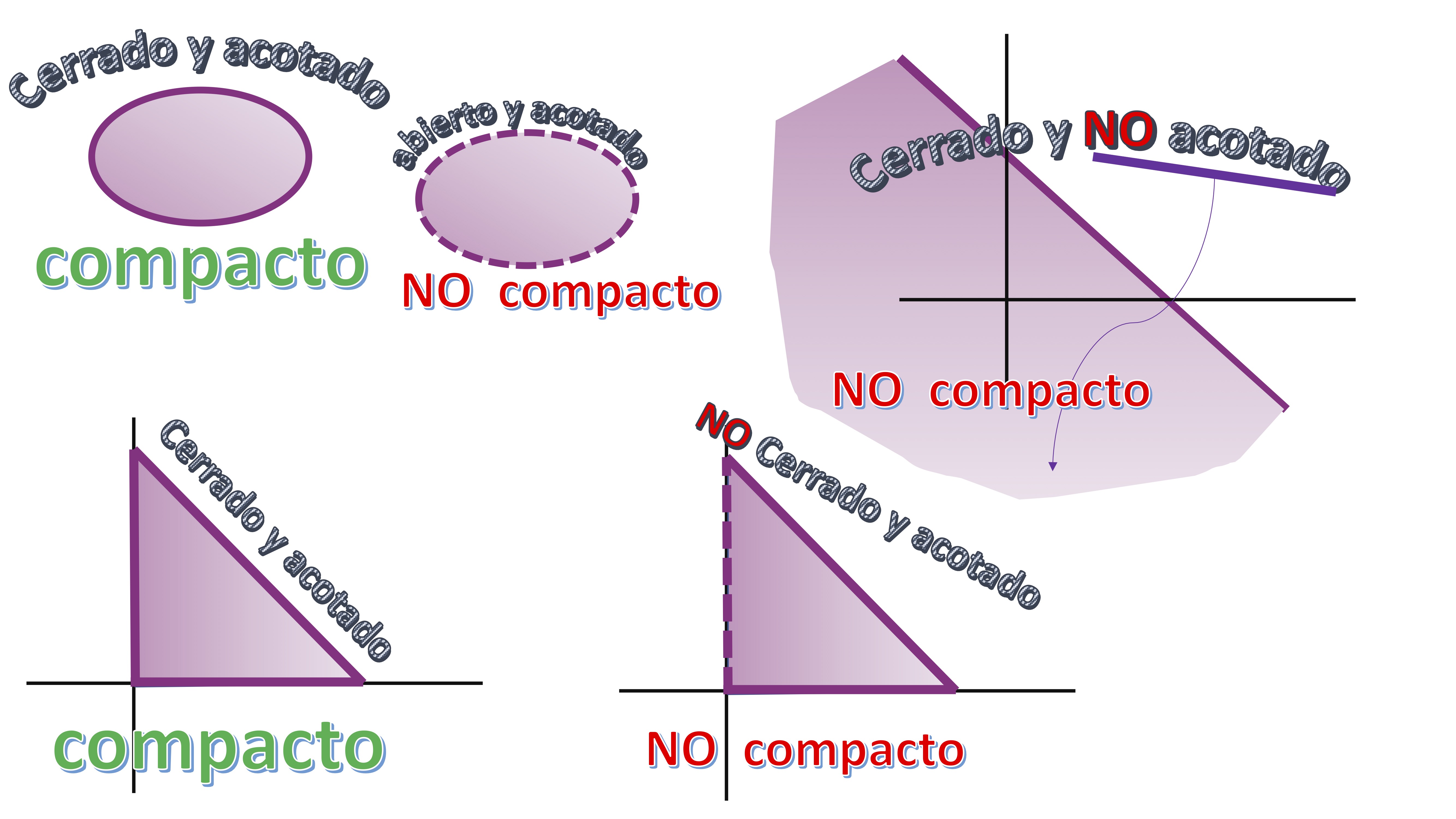
FIG1 compact vs non-compact sets

there is a very celebrated result just when you are working with compact sets (closed + bounded), Weierstrass’s Theorem:

Weierstrass’s theorem If the objective function is continuous in the set of feasible solutions and the set of feasible solutions is compact, the problem has both overall maximum(s) and minimum(s)

---

This is a famous Existence theorem. It does not tell you how to obtain the global maximums/minimums, but it does assure you that these exist under these conditions.

• Example: analyze if you have global optimums in the problem of class #3 and say what they are:

remember:

\[ \mathrm{opt}\:f(x,y)=x^{2}+y \] subject to

\[ \frac{x^{2}}{4}+\frac{y^{2}}{9}\leq1 \]

We analyze the set of feasible solutions. It is an ellipse, as you can remember from the previous year (or high school)

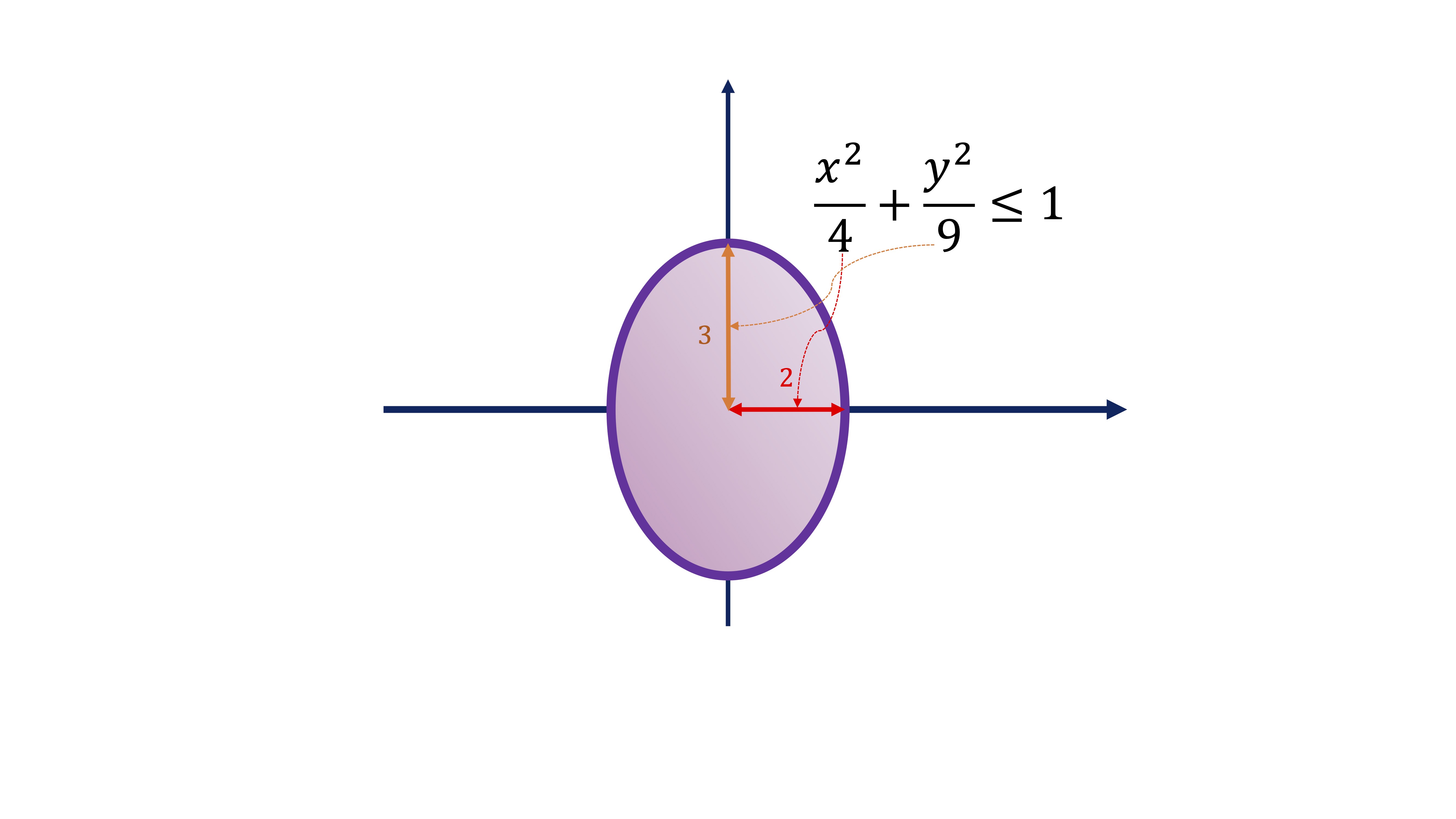as it is closed (the border is included) and bounded (not scattered ek set) then it is COMPACT. This implies that we have global maximum(s) and minimum(s).

-How do we find them? Very easy, let’s go to the leaderboard of the critical points

Point	1	2	3	4
\(x^*\)	0	0	\(\sqrt{55}/4\)	\(-\sqrt{55}/4\)
\(y^*\)	3	-3	\(9/8\)	\(9/8\)
\(\lambda^*\)	3/2	-3/2	\(4\)	\(4\)

and add one more row, where we put the value of the objective function \(f(x,y)=x^2+y\) for each of those points:

Point	1	2	3	4
\(x^*\)	0	0	\(\sqrt{55}/4\)	\(-\sqrt{55}/4\)
\(y^*\)	3	-3	\(9/8\)	\(9/8\)
\(\lambda^*\)	3/2	-3/2	\(4\)	\(4\)
\(f(x^*,y^*)\)	\(3\)	\(-3\)	\(73/16\)	\(73/16\)

So we have to:

• Global minimum: is the point \((x,y)=(0,-3)\)
• Global highs: points \((x,y)=(\sqrt{55}/4.9/8)\) and \((x,y)=(-\sqrt{55}/4.9/8)\)

---

advice!

When you have an optimization problem, the best thing you can do is to first analyze if you check Weierstrass.

Another result: “local-Global” theorem

In addition to Weierstrass’s theorem, we will use another result of interest to search for global points. In this case, the following are sufficient conditions of global maximum-minimum:

GLOBAL Local Theorem If the set of feasible solutions is convex and the objective function is: >- Concave: the candidates for maximum, are maximum global >- Convex: the candidates for minimum, are minimum global

Now, then, we will have to analyze when an objective function is concave or convex and when a set of feasible solutions is convex (beware, there are no concave sets).

In the case of two variables, we will say that a function \(f:\:\mathbb{R}^{2}\rightarrow\mathbb{R}\) is convex if approximated by tangent planes in the environment of a point \((x^{*},y^{*})\), these planes always approximate by default (that is, they are below). On the contrary, it will happen when we want define a concave function: see FIG3:

FIG3 Concave or convex functions

We can use, since the functions with which we will work will behave properly, the following classification criteria:

• STRICTLY CONVEX FUNCTION

If \(f\in\mathcal{C}^{2}\), it will be strictly convex in the set \(X\), if \[ \frac{\partial^{2}f}{\partial x^{2}}>0,\left| Hf(x,y)\right|>0 \]

for all \((x,y)\in X.\) In that case, it will be said that \(Hf(x,y)\) is DEFINED POSITIVE

• STRICTLY CONCAVE FUNCTION

If \(f\in\mathcal{C}^{2}\), it will be strictly concave in the set \(X\), if \[ \frac{\partial^{2}f}{\partial x^{2}}<0,\left| Hf(x,y)\right|>0 \]

for all \((x,y)\in X.\) In that case, it will be said that \(Hf(x,y)\) is DEFINED REFUSAL

• CONVEX FUNCTION

If \(f\in\mathcal{C}^{2}\), it will be convex in the set \(X\), if

\[ \frac{\partial^{2}f}{\partial x^{2}}{\color{red}\geq}0,{\left| Hf(x,y)\right|=0} \]

for all \((x,y)\in X.\) In that case, it will be said that \(Hf(x,y)\) is SEMIDEFINED POSITIVE

• CONCAVE FUNCTION

If \(f\in\mathcal{C}^{2}\), it will be concave in the set \(X\), if \[ \frac{\partial^{2}f}{\partial x^{2}}{\color{red}\leq}0,{\left| Hf(x,y)\right|=0} \]

for all \((x,y)\in X.\) In that case, it will be said that \(Hf(x,y)\) is SEMIDEFINED REFUSAL

Solved Exercise

Check if the following functions are concave or convex

1. \(f(x,y)=-x^{2}-y^{2}\)
2. \(f(x,y)=x^{4}+y^{4}\)
3. \(f(x,y)=x^{2}+y^{2}+2xy\)
4. \(f(x,y)=xy\)
5. \(f(x,y)=y-x^{2}\)
6. \(f(x,y)=2\ln x+\ln y\)

To do this, we need to calculate the Hessian and classify it:

1. \(Hf(x,y)=\left[\begin{array}{cc} -2 & 0\\ 0 & -2 \end{array}\right]\) that meets the condition to be strictly concave. In addition regardless of the value of \(x,y\in\mathbb{R}^{2}\). I mean is strictly concave across its domain (which is \(\mathbb{R}^{2}\))

2. \(Hf(x,y)=\left[\begin{array}{cc} 12x^{2} & 0\\ 0 & 12y^{2} \end{array}\right]\) meets the condition to be convex. If \(x\neq0\) and \(y\neq0\) it will be POSITIVE DEFINED If \(x=0\) or \(y=0\) it will be SEMI-DEFINED POSITIVE (so we do not know, with this criterion, if this function is convex or strictly convex). You can make a drawing in Geogebra and decide it. To do this, look at the environment of \((x,y)=(0,0)\).

3. \(Hf(x,y)=\left[\begin{array}{cc} 2 & 2\\ 2 & 2 \end{array}\right]\) as you can see, it is SEMIDEFINITE POSITIVE, for any value of \(x,y\in\mathbb{R}^{2}\). This indicates that it is convex (but not strictly).

4. \(Hf(x,y)=\left[\begin{array}{cc} 0 & 1\\ 1 & 0 \end{array}\right]\) It does not meet any of the above criteria. We say that the Hessian matrix is INDEFINITE and therefore is neither concave nor convex

5. \(Hf(x,y)=\left[\begin{array}{cc} -2 & 0\\ 0 & 0 \end{array}\right]\) This is SEMI-DEFINED negative. So, we know it’s concave (no strict)

6. \(Hf(x,y)=\left[\begin{array}{cc} -\frac{2}{x^{2}} & 0\\ 0 & -\frac{1}{y^{2}} \end{array}\right]\) This is NEGATIVE DEFINITE. The function is strictly convate

Another result on convexity that interests us is the related with sets. In our case, we will need to be able to analyze feasible sets.

Convex set

We will say that a set is convex if given two points any of the set, the segment that joins them is also within the set

In fact, to identify whether or not a set is convex you must outline it and then see if it meets the definition we have underlining. In the following FIG 4, we can see the idea: in the sets convex, you choose any two points of the set, you trace a segment imaginary and this segment “does not come out” of the whole. That doesn’t happen with nonconvex sets.

FIG4 Convex vs non-convex sets

Examples of convex sets that we will use regularly:

• The space\(\mathbb{R}^{2}\)

• The set of solutions of a linear system of equations (case very concrete of feasible set in our case)

-Intersections of convex sets (eye, not union). Watch this graphic example.

FIG5 Convex vs non-convex sets

Proposed Exercise 6

Analyze what kind of mathematical program we have according to the convexity of this.

• \(\mathrm{opt}\:2x+y,\;s.a\:xy\geq1,x,y\geq0\)
• \(\mathrm{opt}\:(x-1)^{2}+(y-1)^{2},\;s.a\:2x+y\leq10,x,y\geq0\)
• \(\mathrm{opt}\:y-x^{2},\;s.a\:x+y\leq1,x,y\geq0\)
• \(\mathrm{opt}\:x+y,\;s.a\:2x+2y\leq10,x,y\geq0\)

Class 5 The Khun-Tucker method in Excel. Interpretation of the multiplier

Let’s see how, in a simple way, we can get the solution (from global otimo) using the solver tool in Excel. This tool you have to download it from file-options in the case that you have Windows and in tools in the case of that you have Apple.

FIG1 Then, you go to add-ons and from there choose “solver.” Hit “go” and you’ll have to choose “solver” again. You accept, and you already have it

Now let’s work with class 2 problem using Excel. Start by declaring who your variables are, the target function and, of course, restrictions. Do it like this:

FIG2: This is how the problem is written

as you can see, you use it to structure your problem. You must enter which cell is the benefit function, what you want to do with it (max-min), what cells you will modify to get that goal and what restrictions you have.

FIG3: this is specified

if you press “resolve,” you will get this screen. Don’t forget to ask for the sensitivity report:

FIG4: this is specified

Once you request that report, you can analyze which is the optimal (global) that finds Excel and the multiplier. Of course, Excel does not analyze by whether or not the optimum is global. He gives you the best solution. From you it depends on whether we are in the global case analyzing the theorems of sufficient conditions that we have told you!

FIG5: The result

The interpretation of the Lagrange multiplier

Finally, throughout these days you have asked: what do we calculate for? multipliers?

• ANSWER 1: remember that they help us identify if a candidate a solution is for maximum or minimum
• ANSWER 2: it has an interesting economic meaning!!

Imagine that you are facing this problem: \[ \max x^{2}\times y^{2}-x-y \]

s.a

\[ x+y\leq10 \]

\[ x,y>0 \]

You want to analyze, on the other hand, what would happen if these were your Restrictions

\[ x+y\leq{\color{red}11} \]

\[ x,y>0 \]

Let’s calculate the optimal of both problems using Excel:

FIG5: How does the result change?

If we rewrite the problem generically as \[ \max x^{2}\times y^{2}-x-y \]

s.a

\[ x+y\leq{\color{lime}k} \]

\[ x,y>0 \]

If you notice, after changing \(k\) in a unit (\(\triangle k=1)\) the profit goes from 615 units to 904. The difference is 289. That difference is the benefit you could earn, if you produce in a way optimal, by increasing your resources by one unit. That’s called “shadow price.” Imagine that increasing your resource by one unit implies that you must expand your company and the cost of expanding it is 1000 Euros. So, how to expand the company and produce optimally it will only report you 289 euros more, it does not come to account. It is, by both, the maximum amount you would be willing to pay if you do the improvements needed to increase your resources. Well, instead of solve the problem twice, we are going to teach you a way to calculate, approximately, your shadow price. It turns out that the increase in profit in the optimal (or your objective function) can be obtained as \[ \triangle f\simeq\lambda\triangle k \]

It turns out that using differential calculus, we can approximate the value that we expect the target function to be increased. In our case, \[ \lambda=249 \]

(obtained from Excel output). So, as \(\triangle k=1\), we would expect:

\[ \triangle f\simeq249 \]

So, approximately, that is the increase in function objective in the optimal before an increase of the resource. So that it is approximation is good (and, therefore, you do not have to solve the problem for each value of \(k\)), \(\Delta k\rightarrow0.\)