BLOCK 2: Differential Calculus tools

• In this block you will start by remembering (and contextualizing) the derivative. A differential Calculus technique that you have been using for at least two years and that, however, it is difficult for you to define and understand why. Once it is clear, we will take it far, seeing the uses it has.
• Then, it will be time to extend all this artillery to functions of more variables (in general, 2). To do this, you will need to be very clear about the idea of a contour line.

Class 1 (inverted): The derivative

Caution!, inverted class!

This is an inverted class. You should watch the video below and try to think about the exercises that are proposed to you.

The concept of derivative is closely related to the idea of the average rate of variation of a function.

La average rate of change: Let’s imagine that a virus causes a number of infections (in thousands) that is given by the following function \[ y=x^{2} \] where \(x\) is the time measured in months, does this story sound familiar? Its graph will be as follows:

FIG1 Graph with a supposed evolution of the virus.

In such a way that, if we are in month 1, there are a thousand infected and if we are in month 4 there are 16 thousand infected (as you can see in the FIG1). Now, if we want to summarize the information, we can do the following: we take the two points we know \((x_{0},y_{0})=(1,1)\), \((x_{1},y_{1})=(4,16)\) and we can count how many infected average there are per month: what we will call the average rate of variation: \[ TVM=\frac{16-1}{4-1}=5 \] we can, then, say that they have been infected, on average 5000 individuals each month. If you notice, that average rate of variation is calculated the same. that the slope of a straight! Actually, we are calculating the slope of a secant line to the previous curve (i.e. \(y=1+5(x-1)\Rightarrow y=-4+5x\)

FIG2 This is just the secant: try doing it yourself in Geogebra.

Check, now, that you can make many more dryers. All whatever you want!

FIG3 More secants to the curve \(y=x^2\).

the particularity of these dryers is that we are taking, each time, points closest to \((x_{0},y_{0})=(1,1).\) As we approach to that point (which we have chosen as a reference, in the same way that we could have chosen any other) what does the dryer look like?

La instantaneous variation rate: Well, you’ve figured it out. The dryer ends up becoming a tangent. In fact, the slope of the tangent can be found. As you can see, in FIG13, to define the tangent we have to get as close as possible to the point \((x_{0},y_{0}).\) The way we have, in Mathematics, to write that is with a limit. We will say that the slope of the line tangent to the function at the point \((x_{0},y_{0})\) is \[ \lim_{\triangle x\rightarrow0}\frac{\triangle y}{\triangle x} \]

Notice: we use the limit to say that we move very little (a pelín, slightly, etc…) of \(x_{0}\). In order not to call this the slope of the line tangent to the function at the point \((x_{0},y_{0})\), which is very long, we call it DERIVATIVE and write it down as \(y',f',\frac{\mathrm{d}y}{\mathrm{d}x}\) among other notations, in such a way that:

\[ f'(x_{0})=\lim_{\triangle x\rightarrow0}\frac{\triangle y}{\triangle x}=\lim_{\triangle x\rightarrow0}\frac{f(x_{0}+\triangle x)-f(x_{0})}{\triangle x} \]

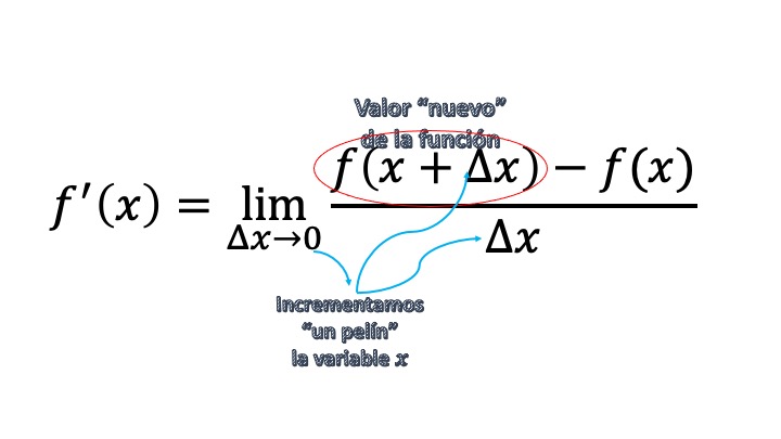
FIG4 We gut the formula.

This definition of derivative will actually allow us to get the usual derivation rules (which are in any book and we ask you to rescue)

Review

On your own the derivatives of the main functions, as well as those derived from composite functions that are solved by the chain rule. This is taken for granted.

Exercise 1

Calculate the derived sifuientes (leaving the result as simplified as possible)

• 1: \(f(x)=\sqrt{2x}-2/x^{2}+\sqrt{3}\),
• 2: \(f(x)=(3x^2-x+2)/x\)
• 3: \(f(x)=\sqrt{2/x}-e^{3}\)
• 4: \(f(x)=1/(2\sqrt{x})\)
• 5: \(f(x)=a^2e^{\sqrt{ax}}+3cos(2x^2-\sqrt{a})\)
• 6: \(f(a)=a^2e^{\sqrt{ax}}+3cos(2x^2-\sqrt{a})\) MirA lA differentiates :)
• 7: \(f(x)=ln{\sqrt{(x^2+1)/(x^2-1)}}\) (you may be interested in applying the properties of the logarithm)

Exercise 2

Calculates \(a.b\) so that the \(f(x)\) function is derivable

\[\begin{equation} f(x) = \begin{cases} a/x & \text{si } x \leq -1 \\ (x^{2}-b)/4 & \text{si } x > -1 \end{cases} \tag{1.2} \end{equation}\]

• Be careful, remember that the tables of derivatives are calculated for a function \(f(x)\), simply put, of “a piece.” Here, we have a “chunks” function so you’ll need to use the definition of derivative, as you’ll have to make the boundaries on the left and right match.

Interpretation of the derivative in Economics

With what we know so far, let’s think:

If I am at the point (1,1) and the derivative of the function is \(f'(x)=2x,\) then the equation of the line tangent to that point will be:

\[ y=y_{0}+f'(x_{0})(x-x_{0}) \]

In this case, \(f'(1)=2,\) so \[ y=1+2(x-1)\Rightarrow y=-1+2x \]

You can see in FIG4 that it is indeed the line tangent to the point (1,1)

FIG4 Here it is clearly seen, using GEOGEBRA that that line is the tangent to the curve at the desired point.

If you notice, in the vicinity of the point (1,1) the curve and the straight they look very similar. Not so with the other dryers traced, right? Let’s go to take advantage of the fact that in the environment of the point (1,1) the tangent line “resembles” the function and we will say that it will be an approximation of the curve in the environment of that point. I mean:

\[ \left.f(x)\right|_{x_{0}}\simeq y_{0}+f'(x_{0})(x-x_{0}) \]

and we read as the function in the environment of the point \(x_{0}\) (so is how \(\left.f(x)\right|_{x_{0}})\) is interpreted is approximately equal to the tangent line. Now, as \(y=f(x),\) we can rewrite the above equation as \[ y\simeq y_{0}+f'(x_{0})(x-x_{0}) \] and, if we pass subtracting \(y_{0},\) then

\[ y-y_{0}\simeq f'(x_{0})(x-x_{0}) \]

As you have already seen, we can write \(\triangle y=(y-y_{0})\), \(\triangle x=(x-x_{0})\) and, therefore, we will have to \[ \triangle y\simeq f'(x_{0})\triangle x \] so that we can say that, if \(\triangle x=1,\) then

\[ \triangle y\simeq f'(x_{0}) \]

I mean:

the derivative is the approximate increment of the \(y\) if we increase \(x\) in one unit.

Please note that the adjective approximate is clearly entered. This is also known as the instantaneous rate of variation to differentiate it from the previous one, which we called tasa of media variation. The adjective instant here it implies increasing “very little” the \(x\).

Siempre we want to analyze how a variable changes when we modify otra, differential calculus is essential. In Economics it is standard to add the adjective “marginal” to the interpretation of a derivative (as you have already seen in Economic Theory). If \(f(x)\) denotes the production of a good, its derivative \(f'(x)\)- which represents the increase in production in the face of a small (marginal) increase in input- is directly interpreted as marginal productivity. Another expression used for the derivative is the concept of rate of variation since it allows us to analyze whether or not the change that occurs in \(f(x)\) is large when increasing \(x\).

Exercise 3

Let \(C(x)=a_2x^2+a_1x+a_0\), with \(a_0,a_1,a_2>0\), the cost function of a company. The good produced is sold at a price \(p>0\) per unit, then the income would be \(R(x)=px\). The profit obtained, if it produced \(x\) units of good would be \(\Pi(x)=R(x)-C(x)\)

• Find the functions of income, cost and marginal benefit
• Determine the value of \(x\) so that the marginal benefit is zero
• Let be \(x=s(p)\), the result obtained in the previous section, calculates the rate of variation of \(x\) if we modify the price in 1 unit.

Class 2 (Magistral): Using the Derivative to Approximate Functions

Have you ever wondered how the computer does this calculation? \[ e^{0.1} \]

you may think that the computer knows to do it in some way I’ll miss that you don’t know. But no: the computer approximates the result using the above idea. As we have seen, if we calculate the line tangent to a curve, we can get a simpler equation that will allow us to approximate the value of a function in the environment of a point. Yes in this case, we take that \(f(x)=e^{x}\) and that, since \(x=0.1\) is close to \(x=0\), we will take that \(x_{0}=0.\) Then, as we already know, \(f'(x)=e^{x}\) and therefore \(f(0)=1,f'(0)=1,\) so \[ \left.f(x)\right|_{x_{0}=0}\simeq1+1(x-0), \]

that is, the function that allows us to approximate \(e^0.1\) is

\[ \left.f(x)\right|_{x_{0}=0}\simeq1+x, \]

in values close to zero (as you already know). So \[ e^{x}\simeq1+x \]

then, \(e^{0.1}\simeq1+0.1=1.1\) (as you can see with the calculator, which makes a better approximation, is not bad at all and has been simple). That yes, only if we use it in the environment of \(x=0.\) Later, we will see how to improve the approach. Watch it in FIG1

You can review this idea in the following Maths & GO video

we can “theorize this idea better.” Look at this figure:

FIG2. The idea of the approximation with the greatest mathematical content.

Where we realize that \(\mathrm{d}y\) is the approximate exchange value of the variable \(y\), if we increase the \(x\) by the amount \(\triangle x\). That increment is calculated as \(\mathrm{d}y=f'(x_0)\triangle x\) and is called “the \(y\) differential.” It is very common to find the differential as \(\mathrm{d}y=f'(x_0)\mathrm{d}x\), where \(\mathrm{d}x=\triangle x\). In our notation, generally, we will prefer the first one and we will say, in addition, that the approximation error we make will be smaller the “smaller” is \(\triangle x\).

What does approximation error mean? Need:

• Realize that \(\frac{\triangle y}{\triangle x}=f'(x)+error\) (i.e., that this quotient—which is the average rate of variation—is equal to the instantaneous rate of variation plus an arbitrary error). It is the same as saying that \(\frac{\triangle y}{\triangle x}\simeq f'(x)\). We change the approximately equal to the equal by adding the error term in the equation.
• \(\triangle y=f'(x)\triangle x+error\triangle x\), si \(\triangle x\rightarrow0\), the error will tend to decrease (faster, since it depends in turn of \(\triangle x,\) as you see in the drawing).
• We will call \(f'(x)\triangle x\) the differential \(\rightarrow\mathrm{d}f(x)\). That is: \(\triangle y\approx\mathrm{d}f(x)\) (or what is the same, we approximate the increase of the variable \(y\) by means of the differential).
• The function at the point is written as \(y_{0}=f(x_{0})\)
• The function at the point at which you want to approximate \(y=f(x)\)
• Entonces, \(\underset{\triangle y}{\underbrace{f(x)-f(x_{0})}}\approx\mathrm{d}f(x)\) if \(\triangle x\rightarrow0\)

A function will be differentiable (which, in our case, we will translate as approximable) if, in this equation,

\[ f(x)-f(x_{0})=\mathrm{d}f(x)+error\triangle x \]

the error tends to zero according to \(\triangle x\rightarrow0\). To do this, in the case of a single variable, what we need is that the function is derivable at the point (or, what is the same, that there is its derivative in that point). So, it is automatically differentiable. So, in functions of a variable, the concept of derivability is identical to differentiability.

Exercise 1

• Approximates, using the idea of video 8, the value of the function \(e^{0.3}\) and \(e^{0.5}\). Make the drawing using geogebra and calculate the mistake you make. Explain the reason for that error. How would you approximate $e^{1.1}?

• Get an approximation of \(\sin0.1\) and \(\cos0.1\). Explain what you would do to get \(\without1.1\) and \(\cos1.1\)

Exercise 2

The production of a good \(y\), depends on the available machines, \(k\), measured in thousands of units, by a function \(y=2k^{1/3}\). Currently $k=$27. Use the linear approximation to:

• calculate the approximate increase in the production of the good if an additional machine is available

• calculate the approximate increase in the production of the good if 1% of additional machines are available.

• calculate the approximate increase in both percent of the good if a thousand additional machines are available.

Second derivatives

A function of a variable, \(f\:\mathbb{R\rightarrow R}\), derivable in a set \(D\subseteq\mathbb{R}\) can support successive derivatives.

For example, the second derivative:

\[ f''(x)=\lim_{h\rightarrow0}\frac{f'(x+h)-f'(x)}{h}, \] as long as the limit exists. Notice that we are calculating the increment on the first derivative, that is, the second derivative, at a point-\(f''(x_{0})-\) comes to indicate how much the first derivative changes (that is, the slope of the tangent line at point \(x_{0})\), if we move slightly on the axis of the \(x\).

If, as we have already seen, \(y=f(x)\) is a production function, \(f'(x)\) measures productivity and, therefore, \(f''(x)\) measures the variation in productivity. In the same way that there may be derivatives of order 2, there can be order \(k\). Notice, if \(f(x)=xe^{x}\), then

\[ f'(x)=e^{x}+xe^{x}=(x+1)and^{x} \]

and, therefore,

\[ f''(x)=e^{x}+e^{x}+xe^{x}=(x+2)and^{x} \]

and, successively

\[ f^{k)}(x)=e^{x}+e^{x}+e^{x}+xe^{x}=(x+k)e^{x} \]

Let’s then, now, try to improve the approaches we have made previously. To do this, we will need the second derivative and, in this way, we will make a quadratic approximation. Watch the video below to motivate the idea

consists, as you have seen in the video, of constructing a second-degree polynomial (using the second derivative) to obtain this expression (which is usually called the second-order Taylor development)

\[ f(x)\simeq f(x_{0})+in (x_{0})(x-x_{0})+\frac{in '(x_{0})}{2}(x-x_{0})^{2}, \]

for this, all we need is for the function to admit, at a minimum, second-order derivatives.

Exercise 3 Repeat the calculations of Exercise 1 but now using this second-degree polynomial. Use Geogebra to make sure you approach the functions much better.

Class 3 (inverted): characteristics of the functions according to \(f'(x)\) and \(f''(x)\)

Caution!, inverted class!

This is an inverted class. You should watch the video below and try to think about the exercises that are proposed to you.

With the first and second derivatives we will be able to classify the behavior of functions \(f\:\mathbb{R\rightarrow R}\). We will attend to growth/degrowth, concavity/convexity and tipping points.

Growth and Degrowth

A function is strictly increasing in an interval \((a,b)\) if when \(x_{1}<x_{2}\), then \(f(x_{1})<f(x_{2}).\) We will say that it is increasing (dry) if it happens that \(f(x_{1})\leq f(x_{2}).\) In the same way, a function will be strictly decreasing in an interval \((a,b)\), if when \(x_{1}<x_{2}\), then \(f(x_{1})>f(x_{2}).\) We will say that it is decreasing (to dry) if it happens that \(f(x_{1})\geq f(x_{2}).\)

• If a function always grows or always decreases we say that it is monotonous.

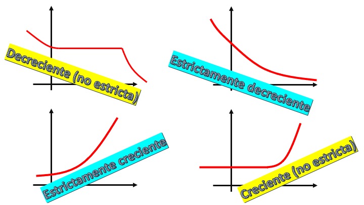
FIG1. A drawing of the definitions we have given.

In FIG1 we can clearly see how to characterize increasing and decreasing functions (strict or not). Using the idea of derivative, in strict increasing functions, the slope is always positive. That is, \(f'(x)>0\). In the increasing (non-strict) the slope is positive or null, that is, \(f'(x)\geq0\). Changing the sign of the derivative is the same with decreasing functions. Therefore, we will say that:

growth/degrowth Caracterización: A \(f(x)\) derivable function: - is increasing in \((a,b)\Longleftrightarrow f'(x)\geq0,\forall x\in(a,b)\) - is decreasing in \((a,b)\Longleftrightarrow f'(x)\leq0,\forall x\in(a,b)\) - is constant in \((a,b)\Longleftrightarrow f'(x)=0,\forall x\in(a,b)\)

From what we get that

• \(f\) is strictly increasing in \((a,b)\Rightarrow f'(x)>0,\forall x\in(a,b)\)

• \(f\) is strictly decreasing in \((a,b)\Rightarrow f'(x)<0,\forall x\in(a,b)\)

If you notice, we have put two distinct symbols in our notation:

FIG2. The implications.

What we intend to say is that, in the first implication, every increasing function in an interval must have a first derivative, in that interval, greater than or equal to zero. This, therefore, includes all kinds of growths (strict and not). In such a way that, in the opposite direction (in the inverse sense of the arrow), it is also fulfilled: if we observe that a function has a derivative greater than or equal to zero then it has to be increasing. The second implication says that strictly increasing functions have to fulfill that their first derivative is, in the interval, strictly greater than zero. It is a sufficient condition: any function that fulfills it, is already automatically strictly increasing. However, this does not operate in the reverse direction. There may be functions that do not satisfy for all \(x\) in the range that \(f'(x)>0\) and yet are strictly increasing. An example: \(f(x)=x^3\). This function is strictly increasing:

FIG3. The typical example of a strictly increasing function with a point where its derivative is null.

but it has a point where \(f'(x)=0\).

The points \(x^*\) where the derivative cancels out (i.e. \(f'(x^*)=0\)), are critical points and can give rise to maximums, minimums (we will talk about it in the optimization block) and inflection points. In the case of \(f(x)=x^3\) we must suspect that it is a turning point, but we still do not know more.

Concavity and convexity

Let be a function \(f(x)\) twice derivable, then

Remember that in the function of a variable \(y=f(x)\), we can define, in the environment of a point \(x_{0}\) the following concepts:

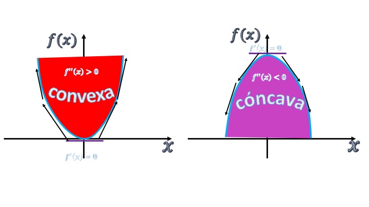
FIG4 Classification of functions of a variable with respect to its convexity/concavity.

A convex function is characterized by the fact that from its minimum point (i.e., with \(f'(x)=0\)) the slopes of the tangent lines on both the right and the left are increasing. As the slopes (i.e. the first derivatives \(f'(x)\)) grow, it is the same as saying that the second derivatives (representing the change of slope at each point) will be greater than zero (\(f''(x)>0\)). In the case of concave functions, the opposite will happen. The slopes (first derivatives) of the tangent lines that start both right and left of the maximum (null derivative) will be decreasing. Again, the second derivative is responsible for modeling the change of the slopes and, therefore, \(f''(x)>0\).

Caution!, the second derivatives

A derivative always measures the change of a function when we increment an input. The second derivative is the derivative of a derivative. Therefore, the second derivative measures the change of the derivative by increasing the input.

In such a way that, looking at FIG4 in this other way, we can analyze two ways of growing and decreasing

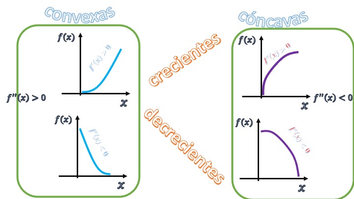
FIG5 We reinterpret growth/degrowth.

• Increasing and convex function: \(f'(x)>0\), \(f''(x)>0\) shows accelerated growth. The higher the $x, the higher the slope of the function. It is equivalent to saying that the function undergoes an acceleration (or accelerated growth) as the $x advances.
• Increasing and concave function: \(f'(x)>0\) and \(f''(x)<0\) presents a cushioned growth. The higher the \(x\), the lower the slope of the function. It is equivalent to saying that it suffers a slowdown (or slowed growth) as the $x progresses.
• Decreasing and convex function \(f'(x)<0\), \(f''(x)>0\) presents a decelerated decrease: the greater the \(x\) the lower the fall of the slope of the function.
• Decreasing and concave function \(f'(x)<0\), \(f''(x)<0\) presents an accelerated decrease: the greater the \(x\) the greater the fall of the slope of the function.

By the way, this analysis has been done with functions that behave muy bien. With somewhat more complicated functions, the idea can be replicated thinking that concave and convex behaviors can occur in environments of specific points of the function.

We will say, in addition

• \(f\) is strictly convex in \((a,b)\Rightarrow f''(x)>0,\forall x\in(a,b)\)

• \(f\) is strictly concave in \((a,b)\Rightarrow f''(x)<0,\forall x\in(a,b)\)

Again, the condition of strict does not operate in both directions. Look at \(f(x)=x^4\). Draw it: it is strictly convex. However, in \(x=0\) its second derivative is zero. Therefore, this condition is sufficient, not necessary.

Exercise Resolved

Let’s use the information to describe a function:

\[ f(x)=x^{3}+x+1 \]

• The first thing that will interest us is to look for the critical points to be able to see what happens in their environments. We get the first derivative \(f'(x)=3x^{2}+1\) and match it to zero.

\[ 3x^{2}+1=0 \]

as we see, it has no critical points, so it is a monotonous function.

• We analyze the first derivative and, as we see, it is always strictly greater than zero, so the function is strictly increasing.

• We analyze the convexity/concavity. With the second derivative, we have to \(f''(x)=6x.\) Let’s see that if \(x>0\), then the second derivative is positive. If $x<0, the second derivative is negative. That is, the function is always increasing, it is convex for \[x>0 and concave for \]x<0. In \(x=0\) therefore has a turning point.

Exercise How would you draw it with this information? Notice that this reduces the number of points in the table of values that we need to compute :).

Exercise 2 Use what you have learned to draw the following functions \(f(x)=x^3\), \(g(x)=3x^5-5x^3\), \(h(x)=\sqrt(x)+2ln(x)\), \(i(x)=\frac{1}{1+x^2}\)

ELASTICITY WEEK

The concept of elasticity is well worth a week: it will be one of the most managed throughout the degree. In many disciplines they will turn to it (marketing, macroeconomics, microeconomics)…. and it is the concept sobre that dudáis the most.

Perhaps, this video will help you to better understand the idea: click on the image

Therefore, elasticity helps us understand ‘’changes’’ (s?, again the idea of the beginning: changes, changes, changes) percentages of the function when the input variable also it changes a bit per cent. For example, in the function

\[\begin{equation} y=f(x),\tag{1.3} \end{equation}\]

we are interested in analyzing the percentage change of the variable \(y\) before a percentage increase of the variable \(x\) and let’s write the linear approximation of (1.3)

\[ \triangle y\simeq f'(x)\triangle x \]

let’s play a little bit now. We will make changes to the equation, but to arrive at another expression in so many percent for both variables. To do this, let’s divide on both sides for \(y\)

\[ \frac{\triangle y}{y}\simeq f'(x)\frac{1}{y}\triangle x, \]

now let’s divide on both sides by \(x\)

\[\begin{equation} \frac{\triangle y}{y}\frac{1}{x}\simeq f'(x)\frac{1}{y}\frac{\triangle x}{x},\tag{1.4} \end{equation}\]

as I want it to stay on the left of the equation (1.4) the change percentage in the \(y\), I pass the \(x\) to the right:

\[ \frac{\triangle y}{y}\simeq f'(x)\frac{x}{y}\frac{\triangle x}{x}, \]

multiplied by 100 on both sides

\[ \left(\frac{\triangle y}{y}\right)\times100\simeq f'(x)\frac{x}{y}\left(\frac{\triangle x}{x}\right)\times100, \]

and I get

\[\begin{equation} \Delta\%y\simeq{f'(x)\frac{x}{y}}\Delta\%x, \end{equation}\]

where \(\Delta\%y\) and \(\Delta\%x\) are read as a percentage cambio of the y and percentage cambio of the x. On the other hand, \({f'(x)\frac{x}{y}}\) is the elasticity. The interpretation, therefore, is clear:

Caution!, elasticity!

if we make \(\Delta\%x=1\), we are increasing the variable \(x\) by 1%. So, if we call \(\epsilon_{y,x}\) the elasticity of the variable \(y\) with respect to the \(x\)

So, \(\epsilon_{y,x}=f'(x)\frac{x}{y}\)

this value indicates the approximate percentage increase of the \(y\) in the face of changes of 1% of the variable \(x\).

Example

If the demand for a good follows the function \(y(p)=\frac{2}{p^{2}}\), the price elasticity (\(\epsilon_{y,p}\)) will be:

\[ \epsilon_{y,p}=\frac{-4}{p^{3}}\frac{p}{y(p)} \]

As you can see, this result is a function. It will depend on the value of the current price. So if, for example, at the moment, the price is $p=$1, the elasticity Be

\[ \epsilon_{y,p}=\frac{-4}{1}\frac{1}{2}=-2 \]

Caution!, we interpret an elasticity!

if I increase the price by 1%,the demand will fall -approximately- by 2%. Don’t forget that elasticity is a percentage concept! Please!

The following content is the work that will be done in the week of elasticity

Class 4 (magistral): Derivatives in functions of \(n\) variables.

Once we have reviewed the most important concepts of derivation, it is time to talk about how we apply this idea in functions of two (or more variables). We introduce the partial derivative, which is another new content in this course.

First, we will try to practice this new type of derivative and, later, investigate its meaning.

A partial derivative of the function \(f(x_1 ,...,x_n)\) consists of deriving the function with respect to the variable \(x_i\) by making the rest of the variables (that is, \(x_{-i}\)) remain constant. That is, if you know how to derive in a variable, this will not cost you

Partial derivatives are usually denoted with the symbol \(\partial\), as you will see below intuitively

We start with a simple function, of two variables, that you have already seen previously (you have seen it in 3D and you have drawn its contour lines, in block 1 of the course).

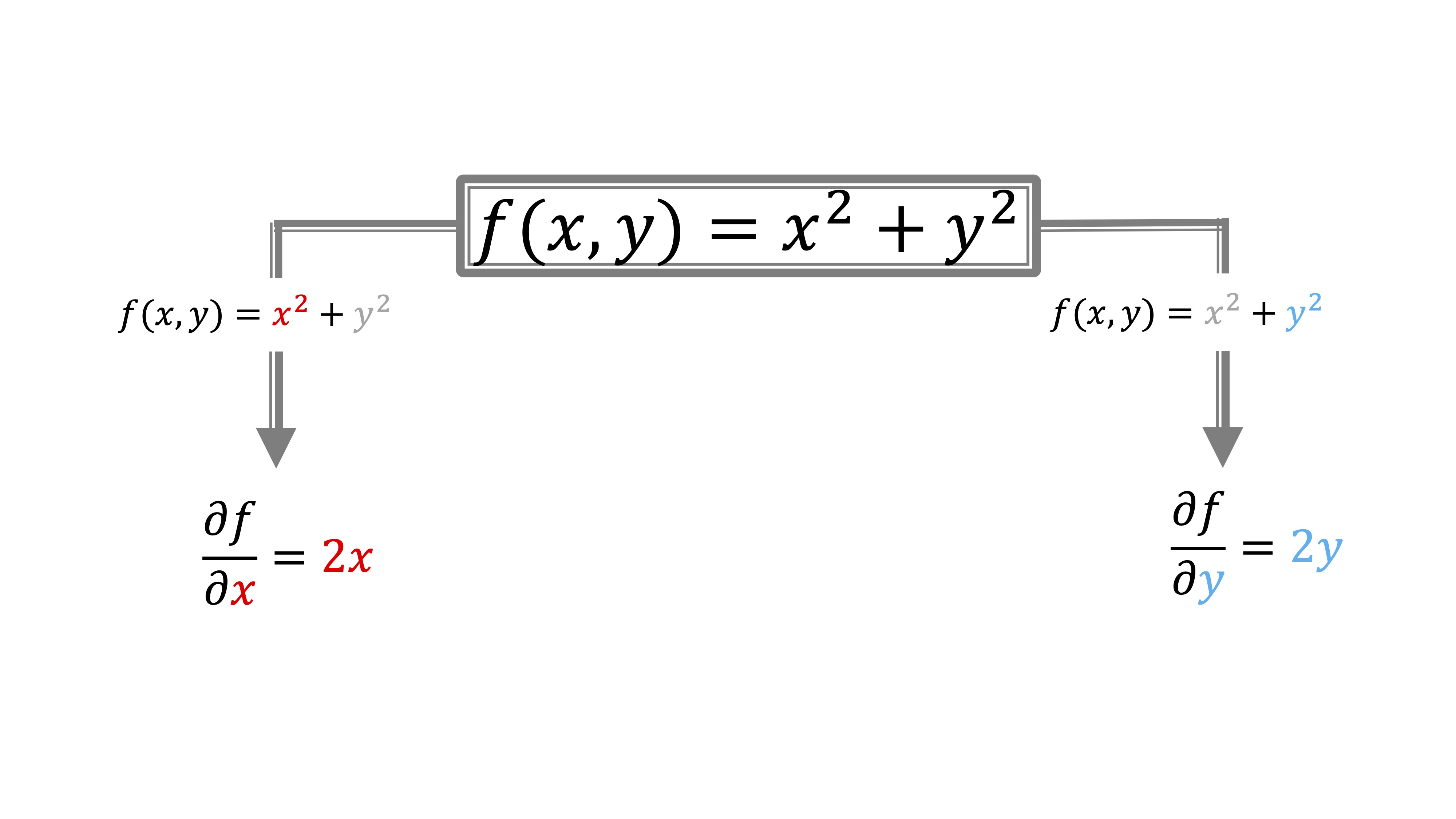
FIG1 The partial derivatives of the function \(f(x,y)=x^2+y^2\)

As you can see, when we derive with respect to \(x\), and write it like this: \(\frac{\partial{f}}{\partial{x}}\) what we are doing is converting the \(y\) into a constant and operate accordingly with the derivation rules. Similarly, when we derive with respect to \(y\). As you can see, I put the \(x\) in red when it is variable and in gray when it is constant: with the \(y\), the same, but in blue.

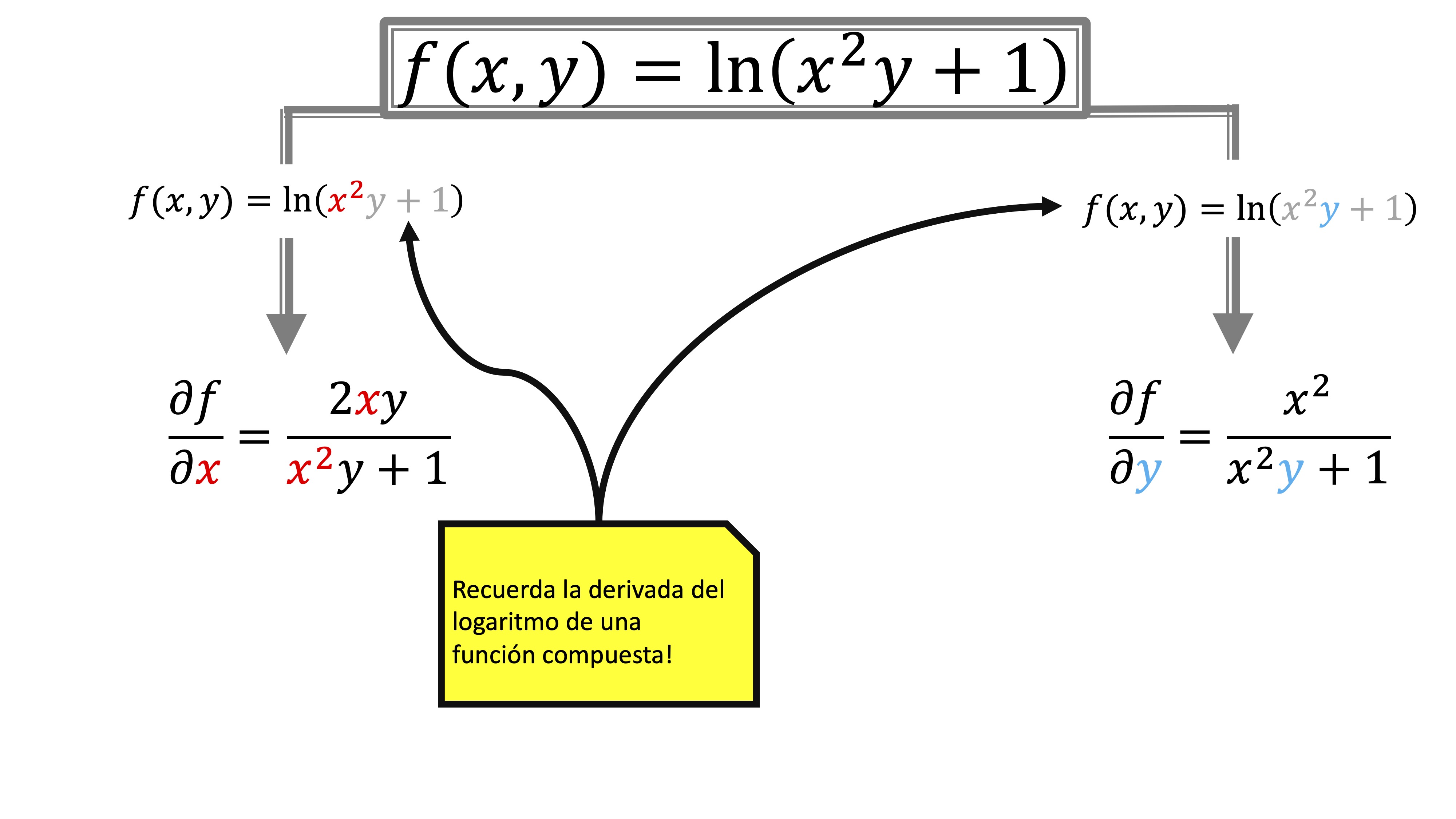
FIG2 The partial derivatives of the function \(f(x,y)=ln(x^2y+1)\)

Now things get complicated: in FIG2 we have a composition of functions: on the one hand, the logarithm, and on the other \(x^2and +1\). Here, to derive, you have to do the same as in a variable. Remember, just in case, what the derivative of the logarithm of a function looks like.

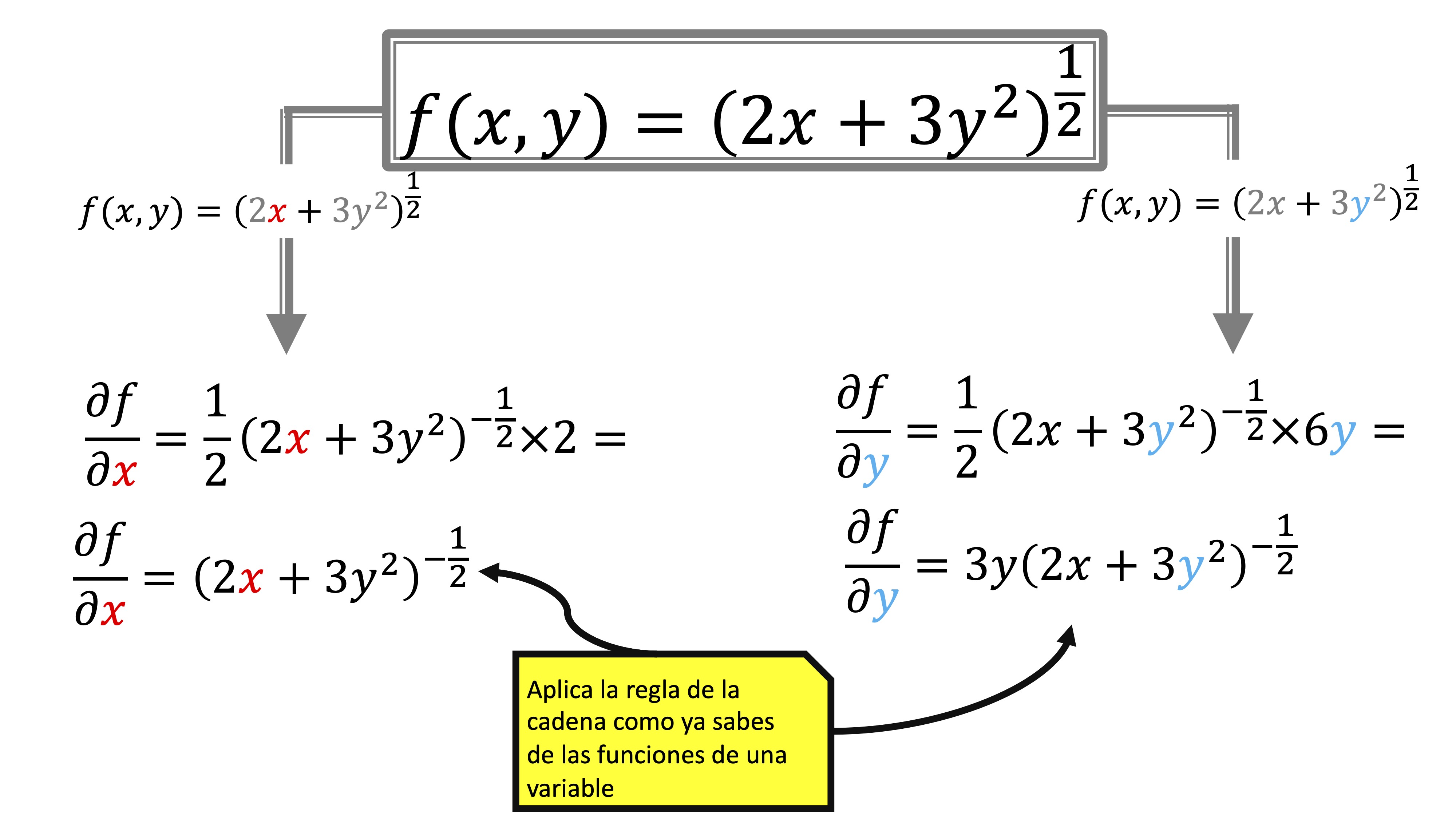And finally, in FIG3 you have the last example: as you will see it is similar to what we have already said.

Exercises solved:

make the following partial derivatives

• \(f(x_{1},x_{2})=x_{1}+6x_{2}^{2}\)

  • \(\frac{\partial f}{\partial x_{1}}=1\)
  • \(\frac{\partial f}{\partial x_{2}}=12x_{2}\)

• \(g(x_{1},x_{2})=\left(x_{1}+6x_{2}^{2}\right)^{2}\) (ten en cuenta the application of the string rule)

  • \(\frac{\partial g}{\partial x_{1}}=2\left(x_{1}+6x_{2}^{2}\right)\)
  • \(\frac{\partial g}{\partial x_{2}}=24x_{2}\left(x_{1}+6x_{2}^{2}\right)\)

• \(h(x_{1}.x_{2})=Ax_{1}^{1/3}x_{2}^{2}\)

  • \(\frac{\partial h}{\partial x_{1}}=\frac{A}{3}x_{1}^{-2/3}x_{2}^{2}\)
  • \(\frac{\partial h}{\partial x_{2}}=2Ax_{1}^{1/3}x_{2}\)

To understand the idea of the partial derivative, let’s start working intuitively with the function, already famous, “paraboloid of revolution” (watch video 2, if you don’t remember it)

\[ y=x_{1}^{2}+x_{2}^{2} \]

that we already drew in 3D and made their contour lines in class 1 and 2. In the graph below, FIG 1, we show some curves level

FIG1 Contour lines of the function \(y=x_1^2+x_2^2\)

As you can see, on the contour lines we have put an arrow (a vector) indicating that we move a unit on the axis of the abscissas and 0 units in the ordered. That is, we increase the variable \(x_{1}\) in a unit and we do not touch the variable \(x_{2}.\) In fact, we have to \(f(0,0)=0,\)y \(f(1,0)=1.\) We can say, by example, that the increment \(\triangle f=f(1,0)-f(0,0)=1.\) Written otherwise that increase: \(f(x_{1}^{0}+\triangle x_{1},x_{2}^{0})-f(x_{1}^{0},x_{2}^{0})\). Notice that we could make calculations similar to those we did with a single variable. We could, therefore, calculate the rate of variation average of the function, before the change that has undergone \(x_{1}.\) Of this form:

\[ TVM_{x_{1}}=\frac{f(x_{1}^{0}+\triangle x_{1},x_{2}^{0})-f(x_{1}^{0},x_{2}^{0})}{\triangle x_{1}} \]

which tells us the average change of the function when increasing \(x_{1}\) and leaving \(x_{2}\) constant (known as ceteris paribus). Now, what if, again, we make \(x_{1}\) as small as we want to leave \(x_{2}\) still?

FIG2 we try to analyze what will happen in the function if we increase \(x_1\) “a crumb.”

As we can see, we will find ourselves in a contour line, marked in blue in FIG2, which has a much smaller value of the function than before. In this way, we can calculate, as with a single variable, the instantaneous rate of variation:

\[ TV{\color{red}I}_{x_{1}}=\lim_{\triangle x_{1}\rightarrow0}\frac{f(x_{1}^{0}+\triangle x_{1},x_{2}^{0})-f(x_{1}^{0},x_{2}^{0})}{\triangle x_{1}} \]

which is to be called derivada parcial. As you can see, it will allow us analyze the impact of a small increase in \(x_{1}\), making \(x_{2}\) unchanged. The partial derivative has its own notation:

Sea function \(f\left(x_{1},x_{2},...,x_{n}\right)\), the derivative partial function with respect to \(x_{i}\) (where \(i\) is cualqueira of possible inputs): \[ \frac{\partial f}{\partial x_{i}} \] or, also, \[ f_{x_{i}}' \]

In the case of a function with two inputs, it is specified in

\[ \frac{\partial f}{\partial x_{1}}=\underset{\triangle x_{1}\rightarrow0}{\lim}\frac{f(x_{1}+\triangle x_{1},x_{2})-f(x_{1},x_{2})}{\triangle x_1} \]

\[ \frac{\partial f}{\partial x_{2}}=\underset{\triangle x_{2}\rightarrow0}{\lim}\frac{f(x_{1},x_{2}+\triangle x_{2})-f(x_{1},x_{2})}{\triangle x_2} \]

Hence, in fact, derivar in a parcial way consists of in leaving constant all the variables with respect to which it is not derived and use the usual derivation rules with the variable \(i\)-th. We gut, for a moment, the formula of the partial derivative

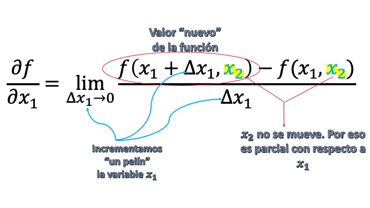
FIG3 … in case it is better understood.

Surely you understand that, in the case of \(x_{2}\) we could make the same visual analysis but, in this case, changing the orientation of the vector \(\overrightarrow{v}.\)

FIG4 The same, but in the direction of the other coordinate axis.

Class 5: More about partial derivatives

As you have seen, we will need to use vectors, in this new chapter. Here is a video where we explain the intuition behind vectors, and some properties that we need you to know.

and this is a small outline with the most important ideas:

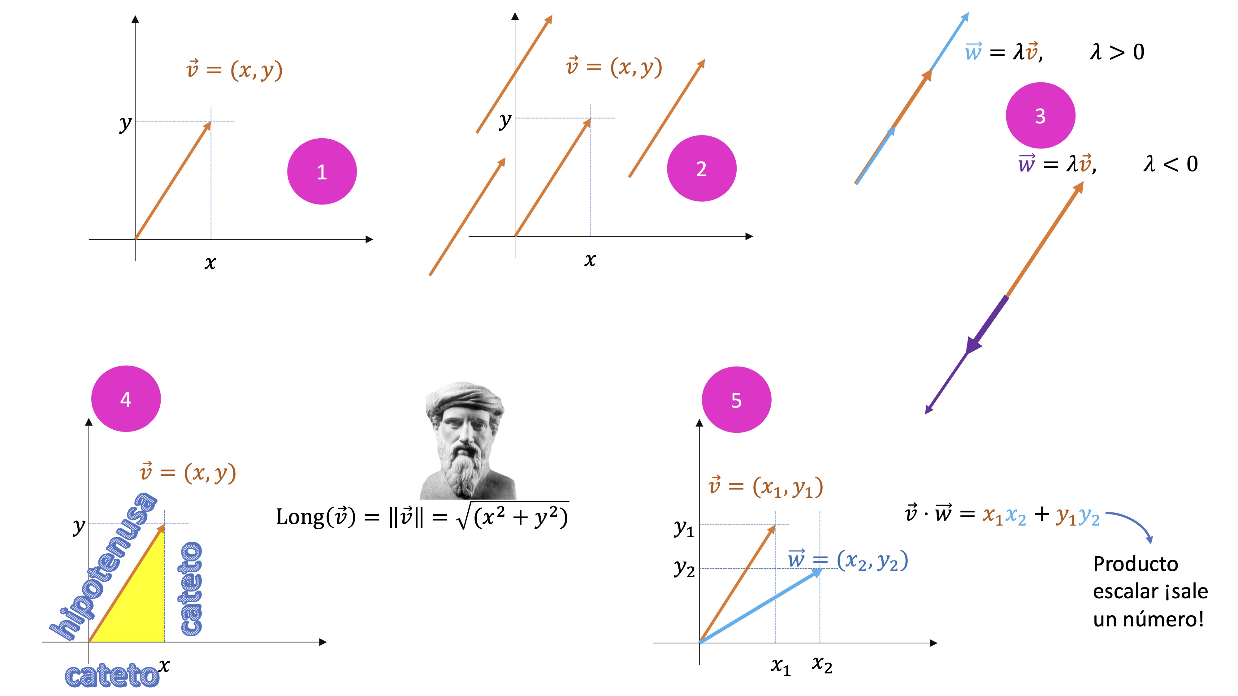
FIG5 Reminder of concepts about vectors that we will need.

• 1. A vector in \(\mathbb{R}^2\) needs two components. It is drawn by joining an arrow from the origin of coordinates to the point determined by the coordinates of the vector.

• 2. But, beware, the same vector can be drawn in any “center” of coordinates we want. The important thing is the direction (and sense): all the vectors drawn are THE SAME.

• 3. If we multiply a vector by a scalar (number), if it is positive, it will have the same direction and the same direction (do not confuse sense with direction). If it is negative it will go in the same direction but in the opposite direction. If \(\lvert{\lambda}\rvert<1\), then the vector will be smaller than the original. Obviously, if \(\lvert{\lambda}\rvert>1\), then the vector will be larger than the original.

• 4. We can calculate “how much it measures” a vector by knowing its coordinates. We call that length “norm” and it is calculated thanks to the Pythagorean Theorem (hypotenuse squared is equal to the sum of the square of its catetos)

• 5. The scalar product of two vectors consists of the sum of the product of the coordinates—in order—of the two vectors. That number gives us a lot of information about the relative position of both vectors: An important result is that if the scalar product of two vectors is ZERO, these vectors are perpendicular

Exercise Let be the vectors \(\vec{v}=(1,2)\) and \(\vec{w}=(2,-1)\),

-a) Draw them starting at point \((1,2)\) - b) Draw the vector \(0.5\vec{v}\), \(2\vec{v}\), \({-2\vec{v}}\), also at the point \((1,2)\) -c) Calculate the length (norm) of the vector How would you find a vector that is proportional to \(\vec{v}\) but has norm 1? - d) Calculate the scalar product of \(\vec{v}=(1,2)\) and \(\vec{w}=(2,-1)\) What do you get? What relationship does it have with what is drawn in (a)?

Let’s go back, now, to the partial derivatives. First, do some Calculus exercises:

Exercise to warm up

Calculates the partial derivatives of the following functions

1: \(f(m,n)=me^{2m-n}\)

2: \(f(x,y)=\frac{xe^{2y+1}}{1+3x}+(y+3)\sqrt{x^{2}+\ln y}\)

3: \(f(p,q)=\ln\left(\frac{p^{2}}{p+q}\right)\)

4: \(f(x,y,z)=xe^{z}\left(\frac{y+x}{z^{2}+1}\right)\)

5: \(f(a,b)=\frac{a}{a+b}+\sin(2a)\)

and now, the goal is to understand the interpretation of a partial derivative. To do this, we will return – again – to talk about the relationship between the average rate of variation and the partial derivative(s) of a function. So far, what we have done is learn the techniques to obtain partial derivatives of functions that are, in turn, functions (unless we derive a linear function). Now let’s see how, evaluating them at one point, we get meaning with economic interpretation.

To continue understanding the idea, let’s look at the case of the mass index let’s remember \(IMC=\frac{p}{a^{2}}\), so that \(p\) is the weight in kilograms and \(a\) is the height in meters of the individual. Now let’s imagine an individual who measures 1.65 meters and weighs 70 kilos (so your BMI is 25.71). The idea of the partial derivative is as follows (FIG1)

• If we do not vary the height (that is, we stay at \(a=1.65\)) we can analyze how BMI changes as weight varies. For example What if we went from weighing 65 kilos to 70?

Let’s calculate, first, the BMI varaition, that is, \(\Delta BMI\), for this:

\[ \Delta IMC=IMC(70,1.65)-IMC(65,1.65)=25.71-23.87=1.84, \]

that is, an individual who goes from \((65,1.65)\) to \((70,1.65)\), increases his BMI by 1.84 points. Now let’s analyze the average variation, that is, for each kilo that increases, how much your BMI increases:

\[ \frac{\Delta IMC}{\Delta p}=\frac{IMC(p+\triangle p, a)-IMC(p,a)}{\triangle p}=\frac{1.84}{5}=0.37 \]

that is, on average, for every kilo that our individual gains weight, his BMI rises 0.37 units.

On the other hand, as we saw, the derivative consists of calculating the previous rate when \(\Delta p\rightarrow 0\). This, in reality, is difficult to interpret. Our imagination does not understand very well what it means that the incremento of the peso is as close as we want to zero, but that it is never zero. However, we will translate it as “how much BMI changes if we increase weight slightly.”

FIG1 The idea of deriving BMI with respect to weight (I leave the height fixed at a value: in this case 1.65), and I move along the weight axis (from 65 to 70 kilos, in this case).

the partial derivative shall be \[ \frac{\partial IMC}{\partial p}=\frac{1}{a^{2}} \] that, evaluated at the point where the individual is

\[ \frac{\partial IMC}{\partial p}(65,1.65)=\frac{1}{1.65^{2}}=0.36 \]

In this case, as you can see, the partial derivative is quite similar to the average rate of variation. This happens because the change that the function has undergone (in this case, gaining 5 kilos) does not seem to be very large. This leads us to say that, if \(\Delta p\) is small enough, then:

\[ \frac{\Delta IMC}{\Delta p}\approx \frac{\partial IMC}{\partial p}(65,1.65) \]

In this way, we can also say that

\[ \Delta IMC\approx \frac{\partial IMC}{\partial p}(65,1.65)\Delta p \]

and, for example, it is normal in economics to attribute as “small” a unit increase in the independent variable (workers, prices, capital, etc …). In this case, it seems sensible, and then, doing \(\Delta p=1\)

\[ \Delta IMC\approx \frac{\partial IMC}{\partial p}(65,1.65)=0.36 \] and, therefore, we will say that the approximate increase in BMI, before changes in one unit of weight, keeping the height constant, when the individual is at the point \((65,1.65)\) is 0.36 units.

However, it is not always true that a unit increase in the independent variable assures us that it is “small” and that, therefore, we can interpret the derivative in this way.

FIG2 Now, the idea of the partial derivative of BMI with respect to height, leaving weight fixed at an arbitrary value.

Imagine an individual who weighs $70 kilos and measures $1.65. Your BMI we already know is $25.71. If he were able to grow a meter, he would measure $2.65 and, keeping the weight constant, his BMI would be $9.96, so he would be $9.96.

\[ \Delta IMC=IMC(70,2.65)-IMC(70,1.65)=9.96-25.71=-15,75, \]

that is, the BMI is reduced by 15.75 units. If we calculate the average rate of variation \[ \frac{\Delta IMC}{\Delta a}=\frac{IMC(p, a+\triangle a)-IMC(p,a)}{\triangle a}=\frac{-15.75}{1}=-15.75, \] as is obvious, for every meter that grows, the BMI falls -in this case- 15.75 units. If we make the partial derivative and evaluate it at the point

\[ \frac{\partial IMC}{\partial a}=\frac{-2p}{a^{3}}, \] I mean

\[ \frac{\partial IMC}{\partial a}(70,1.65)=-31.16, \]

as you can see, the partial derivative and the average rate of variation no longer resemble each other. The partial derivative is overestimating the true variation. In this case, if we wanted to use the partial derivative, we would return to this result:

\[ \Delta IMC\approx \frac{\partial IMC}{\partial a}(70,1.65)\Delta a \]

where \(\Delta a\) should be much smaller than the unit. For example, if the individual grew five centimeters, we would have to

\[ \Delta IMC\approx \frac{\partial IMC}{\partial a}(70,1.65)\times 0.05=-31.16\times 0.05=-1.55 \]

that is, the BMI would be reduced-approximately-by 1.55 units if keeping the weight constant, the individual goes from 1.65 to 1.70. Using the real variation we would obtain:

\[ \Delta IMC=IMC(70,1.70)-IMC(70,1.65)=24.22-25.71=-1.49 \] which, as you can see, now does resemble the derivative.

Then:

• The increase of the function (\(\Delta IMC\), in this case) gives us the exact variation of the function before changes in one of its independent variables
• The partial derivative gives us the approximate variation of the function, before “small” changes in an input leaving the rest constant.
• In Economics, many times, a small change is usually a unit, but not always.
• Partial derivatives are used, for example, to analyze marginal changes in functions (marginal factor productivity, marginal cost, etc…)

You can watch this video from Maths & GO that explains, with the help of the ineffable Homer Simpson, the idea of partial derivative.

Exercise

When \(x\) units of the good are produced \(X\) and \(y\) units of the good \(Y\) costs are incurred given by the function \(C(x,y)=8\sqrt{x^2+3y}\). Currently, $x_0=$2 and $y_0=$4.

1. Calculates the marginal costs (partial derivatives) at any point and at the point \((x_0,y_0)\) and interprets their sign
2. What, approximately, is the variation in the cost if \(x\) is increased by one tenth?
3. What, approximately, is the variation in the cost if \(y\) increases by 10%?

Class 6 The directional derivative and the second derivatives

Now we ask ourselves what if an individual is still in edad of crecer and goes on a diet? Then, not only will it advance in the direction marked by the \(x\) axis or the \(y\) axis, but it will be able to take any direction that will have to be determined, again, with a vector.

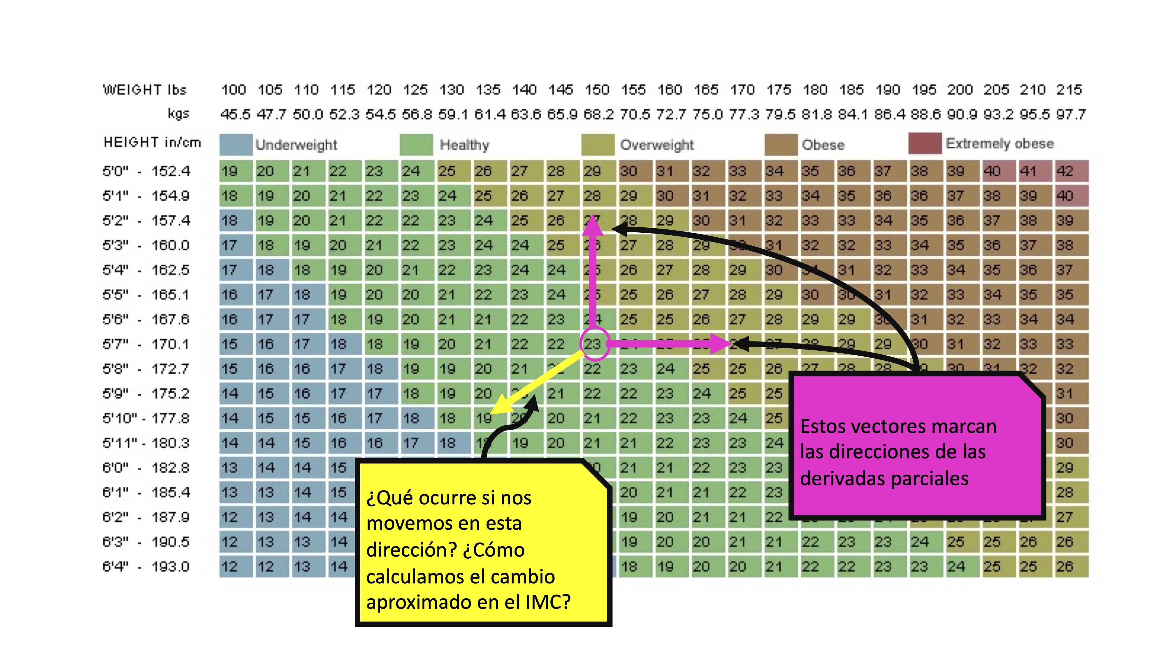Note that, in FIG1, the individual weighs 68.2 and measures 170.1 (therefore has a BMI of 23). If it grows to 177.8 and thins to weigh 61.4, the vector that models that displacement will be: \(\vec{v}=(\Delta weight,\Delta height)=(-6.8,-7.7)\), since it is the change it has suffered in both variables.

A more general case of derivative, therefore, is the directional derivative. This derivative tries to evaluate the increase of the function (in our case \(f(x_1,x_2)\)) when the increments of \(x_1.x_2\) occur in any direction. We will mark the address using “vectors,” so that if the increment vector of both variables is \(\overrightarrow{v}=(v_1, v_2)\), the directional derivative (which will be marked as \(D_\overrightarrow{v}f\)) will simply be

\[ D_\overrightarrow{v}f=\frac{\partial f}{\partial x_1} v_1 + \frac{\partial f}{\partial x_2} v_2 \]

This is usually written, to shorten, as

\[ D_\overrightarrow{v}f=(\frac{\partial f}{\partial x_1} , \frac{\partial f}{\partial x_2})\cdot(v_1,v_2)\]

and this operation is called a “scalar product.”

It is common to use vectors that have norm 1, that is, dividing by the cudrada root of the sum of squares of their components

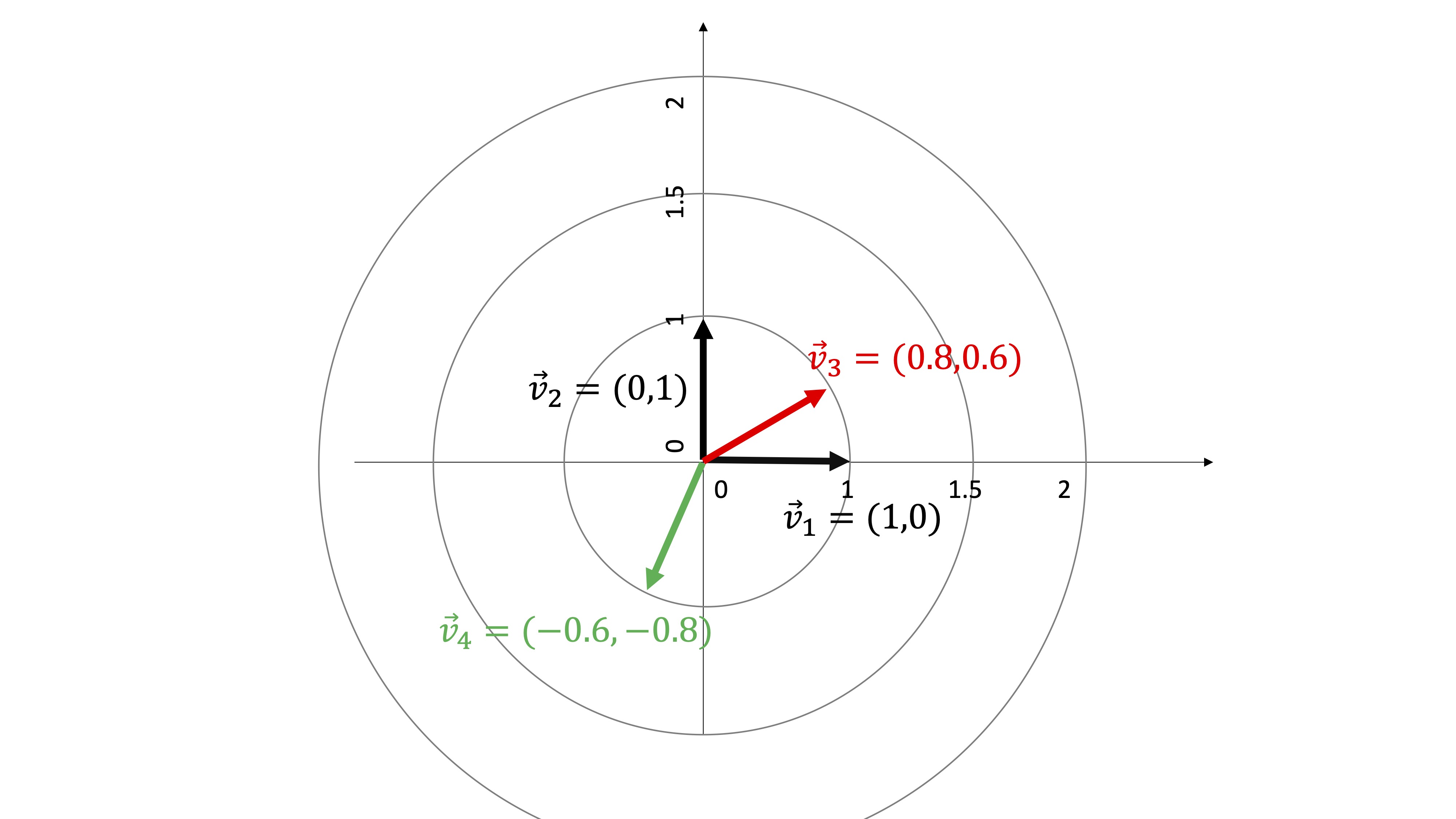
FIG2 Vectors with norm 1 that model the directional derivative

Notice, in this case, all vectors have norm 1. So, let’s look at the following directional derivatives:

• 1. \(D_\overrightarrow{v_1}f=(\frac{\partial f}{\partial x_1} , \frac{\partial f}{\partial x_2})\cdot(1,0)=\frac{\partial f}{\partial x_1}\) It is the partial derivative with respect to \(x_1\)

• 2. \(D_\overrightarrow{v_2}f=(\frac{\partial f}{\partial x_1} , \frac{\partial f}{\partial x_2})\cdot(0,1)=\frac{\partial f}{\partial x_2}\) It is the partial derivative with respect to \(x_1\)

• 3. and (4) \(D_\overrightarrow{v_3}f=(\frac{\partial f}{\partial x_1} , \frac{\partial f}{\partial x_2})\cdot(0.8,0.6)=0.8\times\frac{\partial f}{\partial x_1}+0.6\times\frac{\partial f}{\partial x_2}\) and tells us the rate of variation of the function in the direction of the vector \(\vec{v_3}\). In the same way as \(D_\overrightarrow{v_4}f=(\frac{\partial f}{\partial x_1} , \frac{\partial f}{\partial x_2})\cdot(-0.6,-0.8)=-0.6\times\frac{\partial f}{\partial x_1}-0.8\times\frac{\partial f}{\partial x_2}\) and tells us the rate of variation of the function in the direction of the vector \(\vec{v_4}\).

Exercise With Homer Simpson data, get the following results:

• The partial derivative of BMI with respect to weight and height. Interpret its meaning
• The directional derivative if you decide to advance in the direction “for every kilo that I gain I grow a centimeter.” Interpret the result
• What if it were in the opposite direction, that is, for every kilo that I lose weight I decrease one centimeter? (don’t forget it’s a cartoon: it can grow and decrease as it wants)

Second partial derivatives

In the same way as with the functions of a variable, the variable \(n\) functions also have second, third derivatives, etc… whenever it is possible to continue drifting.

Caution!, we interpret the first partial derivatives, geometrically, of a function \(f(x,y)\)

As in the case of a variable, the first partial derivatives of a function inform us whether the function is increasing or decreasing with respect to the variable with which we derive, keeping the other constant(s).

Example Let be the function \(f(x,y)=e^{-x}/y^2\) Is the function decreasing with respect to \(x\) and \(y\) for any \((x,y)\)? In FIG3, you can observe the function in the 3D graph (yes, to understand this concept we are going to ask you to look at 3D graphics)

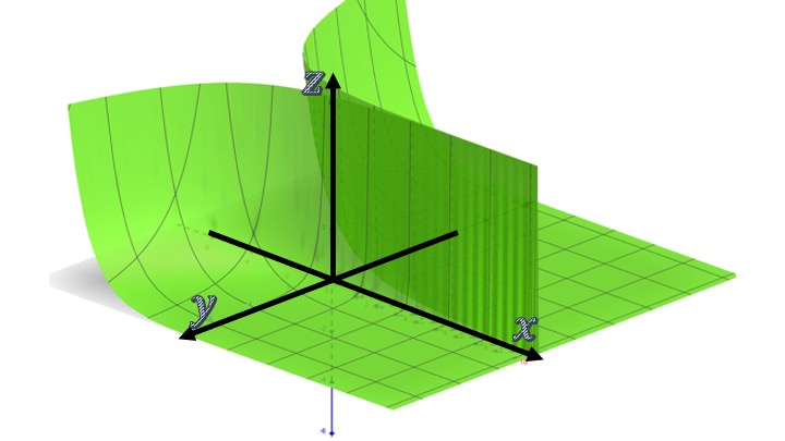
FIG3 The function \(f(x,y)=e^{-x}/y^2\).

To do this, we obtain the first partial derivative with respect to \(x\) and \(y\)

\[ f'_{x}=\frac{-e^{-x}}{y^2}. \]

in this case, for any value of \((x,y)\) the partial derivative with respect to \(x\) is negative. That means that, if we look at the function, ignoring the axis of the \(y\), the profile of this will be that of a decreasing function. You can see it in FIG4, as the \(x\) grows, the \(z\) decreases.

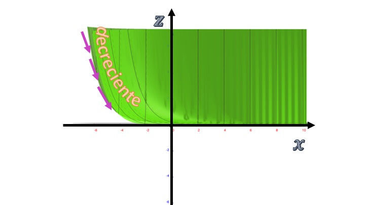
FIG4 We rotate the function \(f(x,y)=e^{-x}/y^2\) to see the idea of the partial derivative with respect to \(x\).

On the other hand

\[ f'_{y}=\frac{-2e^{-x}}{y^3}. \]

As we can see, the numerator is always negative for any \(x\). The denominator is negative for \[y<0 and positive for \]y>0. Therefore, for any value of \(x\), the ratio between \(z\) and \(y\) will be increasing if \(y<0\) and decreasing if \(y>0\). You can see in FIG5 how, indeed, by “forgetting” the axis of the “x” and analyzing the relationship between \(z\) and \(y\), we see the increasing and decreasing function.

FIG5 We rotate the function \(f(x,y)=e^{-x}/y^2\) to see the idea of the partial derivative with respect to \(y\).

Remember that in the function of a variable \(y=f(x)\), we can define, in the environment of a point \(x_{0}\) the following concepts:

• A convex function is characterized by the fact that from its minimum point (that is, with \(f'(x)=0\)) the slopes of the tangent lines both to the right and to the left are increasing. As the slopes (i.e. the first derivatives \(f'(x)\)) grow, it is the same as saying that the second derivatives (representing the change of slope at each point) will be greater than zero (\(f''(x)>0\)).

• In the case of concave functions, the opposite will happen. The slopes (first derivatives) of the tangent lines that start both right and left of the maximum (null derivative) will be decreasing. Again, the second derivative is responsible for modeling the change of the slopes and, therefore, \(f''(x)>0\).

Caution!, the second derivatives

A derivative always measures the change of a function when we increment an input. The second derivative is the derivative of a derivative. Therefore, the second derivative measures the change of the derivative by increasing the input.

In such a way that, as you already know from the Calculus in a variable, there are two ways to grow and decrease

• Increasing and convex function: \(f'(x)>0\), \(f''(x)>0\) shows accelerated growth. The higher the $x, the higher the slope of the function. It is equivalent to saying that the function undergoes an acceleration (or accelerated growth) as the $x advances.
• Increasing and concave function: \(f'(x)>0\) and \(f''(x)<0\) presents a cushioned growth. The higher the \(x\), the lower the slope of the function. It is equivalent to saying that it suffers a slowdown (or slowed growth) as the $x progresses.
• Decreasing and convex function \(f'(x)<0\), \(f''(x)>0\) presents a decelerated decrease: the greater the \(x\) the lower the fall of the slope of the function.
• Decreasing and concave function \(f'(x)<0\), \(f''(x)<0\) presents an accelerated decrease: the greater the \(x\) the greater the fall of the slope of the function.

By the way, this analysis has been done with functions that behave muy bien. With somewhat more complicated functions, the idea can be replicated thinking that concave and convex behaviors can occur in environments of specific points of the function.

Now, applying this in a function with n variables, we will have two types of second partial derivatives. Let’s assume a function \(z=f(x,y)\)

La second derivative with respect to the same variable

\[ \frac{\partial^{2}f}{\partial x^{2}}\left(x_{0},y_{0}\right) \]

which represents the change of the slope of the function with respect to the axis of the \(x\), being at the point \((x_{0},y_{0}).\) and leaving the variable \(y\) fixed. It allows us to analyze the concavity, convexity of the function in the direction of \(x\) (i.e. leaving fixed \(y=y_0\). Also it is written \(f''_{xx}(x_{0},y_{0}).\)

In the example we are working with, we will have to

\[ f''_{xx}=\frac{e^{-x}}{y^2}. \]

that will always be positive. This means that the slopes of the function with respect to the axis \(x\) will be increasing and that, therefore, leaving the axis fixed \(y\), the profile of the function will be convex:

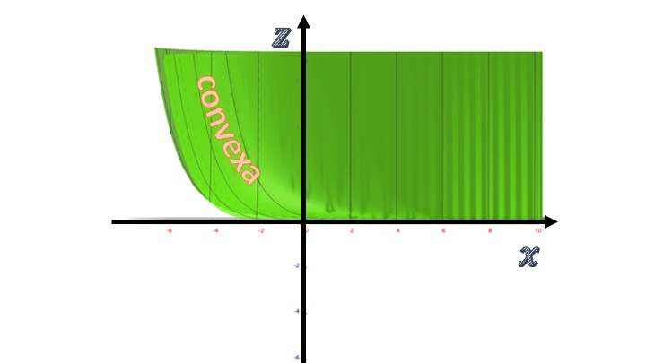
FIG6 We now analyze the convexity/concavity of the function with respect to the axis of the \(x\).

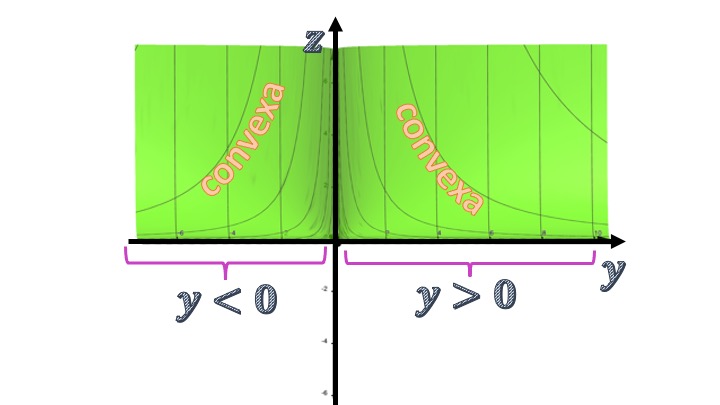
FIG7 We now analyze the convexity/concavity of the function with respect to the axis of the \(y\).

On the other hand

\[ f''_{yy}=\frac{6e^{-x}}{y^4}. \]

in such a way that, for any value of \(y\) the second derivative is positive and, therefore, the function, if we forget the axis of the \(x\), will have a convex function profile by relating the axis of the \(y\) with that of \(z\).

Caution!, the function has been chosen to make it easy to “forget” the axis of the \(x\) and that of the \(y\). In more complicated functions it is not so easy to see graphically, since the concavity / convexity may depend on the value of the other variable

Caution!(2): if you have trouble seeing it in the graph I recommend that you try to make the drawing in Geogebra and navigate through the function trying to calmly see all the details. If, even so, it is not possible for you: RELAX!, geometric arguments only try to help by illustrating concepts: but it is not the only way to learn

La second derivative with respect to another variable (second cross derivative)

We write it this way:

\[ \frac{\partial^{2}f}{\partial x\partial y}\left(x_{0},y_{0}\right) \]

representing the change of the partial derivative with respect to the \(x\), that is, \(\frac{\partial f}{\partial x}\) by increasing the variable \(y\), being at the point \((x_{0},y_{0}).\) It is a way of analyzing cross-effects of a variable on the changes in the function provided by the other variable. It is also written as \(f_{xy}(x_{0},y_{0}).\)

That is, we must take the partial derivative with respect to \(x\) and, now, derive it with respect to \(y\):

\[ f''_{xy}=\frac{2e^{-x}}{y^3}. \]

which tells us:

• if \(y<0\), the slope \(f'_x\) will decrease with the \(y\) (as you can see in the drawing: different slope profiles at a point of \(x\) for different values of \(y\))
• If \(y>0\), the slope \(f'_x\) will grow with the \(y\) (that is not much appreciated in the graph).

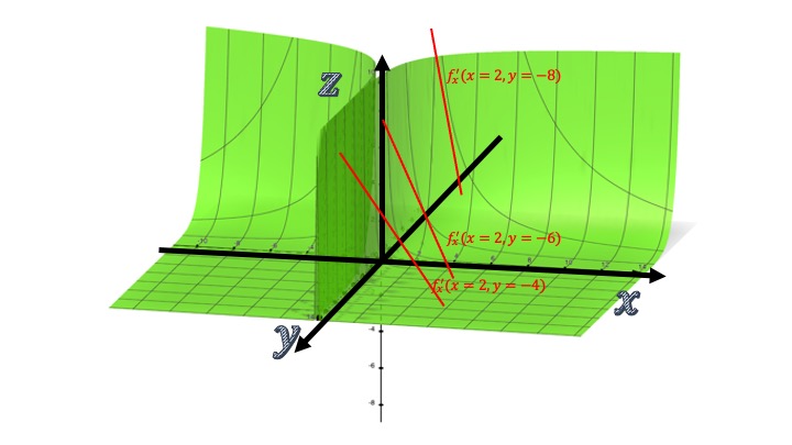
FIG8 We now analyze how \(f'_x\) evolves for different values of the \(y\)

On the other hand, we have that if we derive with respect to \(x\) the derivative that we already had with respect to \(y\):

\[ f''_{yx}=\frac{2e^{-x}}{y^3}. \]

• if \(y<0\), the slope \(f'_y\) will decrease with the \(x\)
• If \(y>0\), the slope \(f'_y\) will grow with the \(x\)

Important note: The cross partial derivatives are the same! Will this always be so? And

Schwartz’s theorem

in functions with derivadas second continuas crosses defined in your domain of \(\mathbb{R}^{n}\), the second cross derivatives serán simétricas:

\[ \frac{\partial^{2}f}{\partial x_{i}\partial x_{j}}=\frac{\partial^{2}f}{\partial x_{j}\partial x_{i}} \] \(i \neq j\)

The functions we are going to work with in this course ALWAYS will verify Schwartz’s Theorem

On the other hand, we will need two instruments to store the information we are capturing from the functions. Define the gradient vector of the function \(f(x_{1},...,x_{n})\) to a vector in \(\mathbb{R}^{n}\) such that

\[ \nabla f(x_{1},...,x_{n})=\left[\frac{\partial f}{\partial x_{1}},...,\frac{\partial f}{\partial x_{n}}\right] \]

That is, it is denoted \(\nabla\) (not to be confused with the increment sign). You see, for now, all we need to know about the gradient is that it is a vector… (again) In this vector, we enter in an orderly way partial derivatives. For example, from the function \(f(x,y,z)=x^{2}y+z\), this is the gradient vector:

\[ \nabla f(x,y,z)=\left[2xy,x^{2},1\right]. \]

On the other hand, the second partial derivatives, we will introduce them in… a MATRIX! Yes, remember that, for now, a matrix is the form more elegant than we know to store information. Well we will define the Hessian matrix of the function \(f(x_{1},...,x_{n})\) to a matrix of real numbers of dimension \(n\times n\) such that

\(Hf(x_{1},...,x_{n})=\left[\begin{array}{cccc} \frac{\partial^{2}f}{\partial x_{1}^{2}} & {\frac{\partial^{2}f}{\partial x_{1}\partial x_{2}}} & ... & \frac{\partial^{2}f}{\partial x_{1}\partial x_{n}}\\ \frac{\partial^{2}f}{\partial x_{2}\partial x_{1}} & \frac{\partial^{2}f}{\partial x_{2}^{2}} &... &...\\ ... &... &... &...\\ \frac{\partial^{2}f}{\partial x_{n}\partial x_{1}} &... &... & \frac{\partial^{2}f}{\partial x_{n}^{2}} \end{array}\right]\).

Exercise Write the expression of a directional derivative of the function \(f\) using the gradient, the displacement vector \(\vec{v}\) and the scalar product.

Class 7 Practice of everything learned so far

From ELASTICITY WEEK, you learned the concept focused on functions of a variable. In the event that we have a function of more than one variable, everything it remains very similar. In this case, the function will be:

\[ y=f(x_{1},x_{2},...,x_{n}) \]

in such a way that if you want to analyze the marginal change in so many percent of \(y\) in the face of changes in so many percent of anyone of the variables \(x_1,... x_n\), keeping the rest constant, you must do the following:

\[ \triangle\%y\simeq\underset{\varepsilon_{y,x_{i}}}{\underbrace{\frac{\partial f}{\partial x_{i}}(x_{1},...,x_{n})\frac{x_{i}}{f(x_{1},...,x_{n})}}}\triangle\%x_{i} \]

where \(i=1,..,n\). That is, as you can see, you just have to change the derivative by the partial derivative of any of the possible \(x_i\) that compose the function and use the same formula. We will have, then, la elasticity parcial since we must not forget that the rest of the inputs of the function have not been modified. For example in the function:

\[ y=3x_{1}^{2/3}x_{2}^{-1/2} \]

if we want to obtain the partial elasticity of the first variable when \(x_{1}=8\) and \(x_{2}=1,\) we will do the following

\[ \varepsilon_{y,x_{1}}=\frac{\partial f}{\partial x_{1}}(x_{1},x_{2})\frac{x_{1}}{f(x_{1},x_{2})}=\frac{2}{3}3x_{1}^{-1/3}x_{2}^{-1/2}\frac{x_{1}}{3x_{1}^{2/3}x_{2}^{-1/2}}=2/3 \]

This implies that, if we increase \(x_{1}\) by 1%, the \(y\) will increase, approximately 0.66%, that is:

\[ \triangle\%y\simeq2/3. \]

Exercise 1

Let \(f(x,y)=\frac{2x^2}{3x^2-y}\), find and interpret the partial elasticity with respect to \(x\) at the point \((x_0,y_0)=(2,4)\).

Exercise 2 The quantity demanded of a certain good with a price \(p\) by a consumer with income \(m\) is given by the function \(f(p,m)=\frac{6m}{(1+p)p}\)

1. Calculates the partial derivatives of the function at any point \((p,m)\) and interprets its sign
2. Calculates the elasticity of the function with respect to any point \((p,m)\). Is it true that if \(m\) increases by \(3%\) the demand increases by \(3%\)?

Exercise 3

The profits of a company depend on the price per unit of capital \(r\) and the price per unit of work \(w\) according to a function \(\varPi(r,w)\) of which we know its gradient \(\nabla\varPi(r,w)=(\frac{-100}{r^{2}},\frac{-100}{w^{2}})\) y su Hessiana \(H\varPi=\left[\begin{array}{cc} \frac{200}{r^{2}} & 0\\ 0 & \frac{200}{w^{2}} \end{array}\right]\).

Reason if it is true that:_ the variation in profit, as it increases r, is in absolute value, higher the higher is \(r\)_

Exercise 4

Calculates the gradient of the function \(f(a,b)=\frac{3a+2b^{2}}{\sqrt{2a+1}}\) at the point \((a_{0},b_{0})=(0,4)\) and interprets the sign of its Components.

Exercise 5

Let \(f(L,K)\) the amount of product obtained using \(L\) units of work and \(K\) units of capital. Currently $f(120.20)=$240 and \(\nabla f(120,20)=(3,2).\) Say, justifying your answer, if they are true or the following statements are false: a) If \(4%\) of the workers are fired, the amount of product will be dismissed. reduce un \(6\%.\) b) If \(K\) is increased by \(2\%\) the amount produced is approximately 240.04 units.

Exercise 6

Demand $x of butter (in tons) is a function of the price \(p\) of the kilo of butter and the price \(q\) per kilo of margarine (both prices are given in euros). Currently, prices are \(p_{0}\) and \(q_{0}\) and the demand is \(x_{0}.\) Express, using first partial derivatives and/or second or elasticities the following facts:

1. The demand for butter increases as the price of margarine increases, and this increase is greater the lower the price of butter.

2. If the price of butter increases by \(2\%\) the demand for butter decreases by approximately \(4\%.\)

3. If the price of butter increases by 20 euro cents per kilo, then the demand for butter decreases by approximately 100 Kg.

Exercise resolved

The quantity produced of a certain good is given by the function \(y=f(L,K)=4L^{1/2}K^{\beta },\) \(\beta >0.\) Halle, if possible, all values of the $$ parameter so that: a) The function \(\partial f/\partial K\) is decreasing by \(K.\) b) The function \(\partial f/\partial L\) is increasing by \(K\) and decreasing by \(L.\) c) The function \(\partial f/\partial K\) is decreasing by \(L\) and the function \(\partial f/\partial L\) is increasing by \(K.\)

solution

The partial with respect to \(K\) is \(f_{K}^{\prime }=4\beta L^{1/2}K^{\beta -1}\)

1. This partial is decreasing by \(K\) if when deriving it with respect to \(K\) the derivative is negative

\(f_{KK}^{\prime \prime }=4\beta (\beta -1)L^{1/2}K^{\beta -2}\) which is negative if \(0<\beta <1.\)

2. For \(\partial f/\partial L\) to be increasing by \(K\) \(f_{LK}^{\prime \prime }>0\) must be met and for it to be decreasing by \(L\) \(f_{LL}^{\prime \prime }<0\) must be met. Since \(f_{L}^{\prime }=2L^{-1/2}K^{\beta }\) you have

\(f_{LK}^{\prime \prime }=2\beta L^{-1/2}K^{\beta -1}\) \(f_{LL}^{\prime \prime }=-L^{-3/2}K^{\beta }<0\)

luego \(\beta >0.\)

3. It should be fulfilled \(f_{KL}^{\prime \prime }<0\) and \(f_{LK}^{\prime\prime}>0\) which is impossible because the function \(C^{2}\) is the theorem of Schwartz says the partial cross derivatives must be equal.

Class 8: The linear approximation

Exercise to warm up Let \(B(K,L)\) be the function that provides the benefits of a company that employs \(K\) units of capital and \(L\) units of work. It is known that $B(2.8)=$10 and that \(\nabla B(2,8)=(3,-2)\), say if the following statements are true in the point \((2,8)\):

1. The employer, counting on the current capital, should hire more workers if he wants to increase the profit
2. A variation in profit of 3 hundredths is a percentage change in profit of \(3\%\)
3. If the capital is increased by \(2\%\), the profit increases by approximately 0.06 units
4. The profit function is elastic with respect to \(K\) at the point \((2,8)\)

Remember that, in functions of a variable, we use the line tangent to a point as the function simpler that allows us to approximate a complicated function (remember that, for example, we saw that if I want to get the value for $x=$0.1 of \(f(x)=e^{x}\) about \(x=0,\) we use approximately \(f(x)\simeq1+x,\) that is, \(e^{0.1}\simeq1.1).\) Remember, therefore, that:

Diferenciabilidad of a function in a variable: \(f\) is a differentiable function in the \(x_{0}\) environment if the Approximation error is made as small as possible when \(\triangle x\rightarrow0\).

In functions of a variable, if the derivative exists at a point (that is, the function is derivable at that point), we can approximate it in the environment of that point and, therefore, we will automatically say that it is differentiable (and, therefore, continuous and without peaks). For variable $n functions, this is not automatic.

To see what we are going to do, we put the immediate translation in two variables of what you already knew how to do with a function in a variable

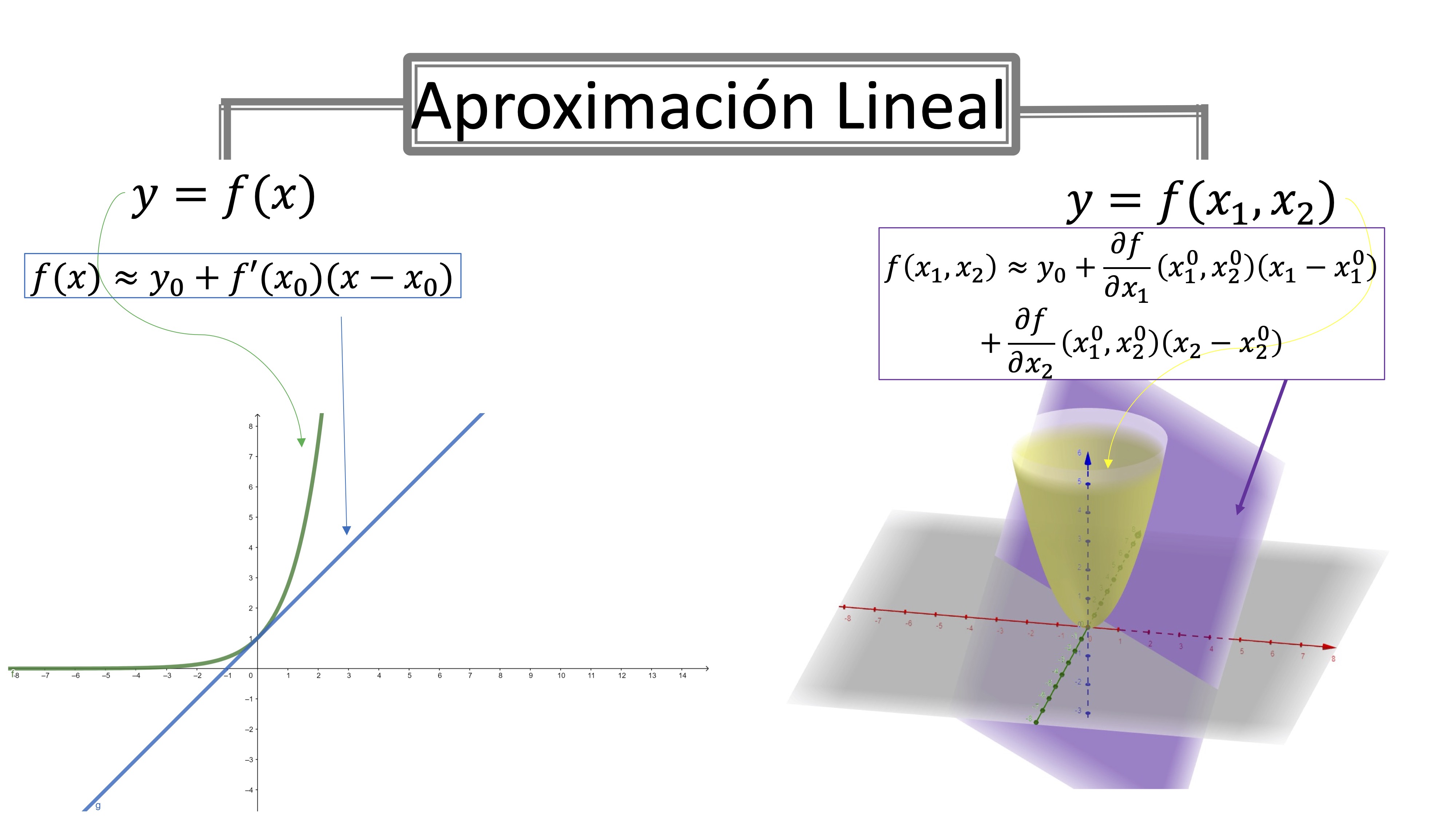
FIG1. A comparison in 1 variable and 2 variables

The approximation of functions \(\mathbb{R}^{2}\rightarrow\mathbb{R}\)

In order to take this concept to functions of two variables we must, first- as you have seen in FIG1- review the equation of the plane in \(\mathbb{R}^{3}\).

Would you know what the equation of a 3D plane that goes through the points \((0,0,0)\)?

\[ z=ax+by \]

It is normal to write it as a function of two variables:

\[ z=f(x,y)=Ax+By \]

if we go to google and type “z=3x-2y,” then we get:

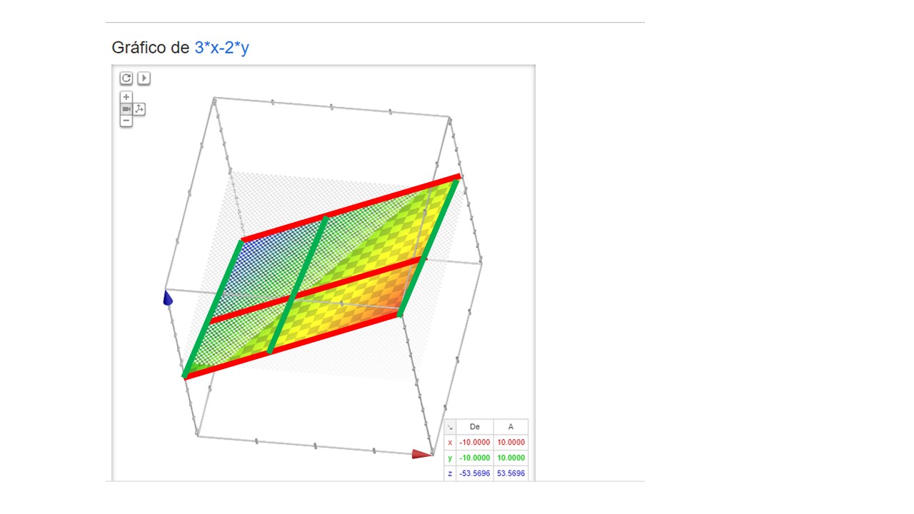
FIG2. The equation of the plane that Google gives us.

In fact, in general, a plane that passes through an arbitrary point in \(\mathbb{R}^{3}\) : \(\left(x_{0},y_{0},z_{0}\right)\) it is written as:

\[\begin{equation} z-z_{0}=A\left(x-x_{0}\right)+B\left(y-y_{0}\right)) \tag{1.5} \end{equation}\]

Let’s think now:

What are \(A,B?\)?

son slopes of the plane: Then, as we want to approximate the function \(f(x,y),\) in a similar way as we did in functions of a variable, now we will use-instead of a line- a plane to make such aprocimación. How do we search for \(A.B\)?

Let’s think with what we already know about derivatives and partial derivatives:

If I freeze the axis \(y\), then I move around the axis of the \(x\).}

\[ z-z_{0}=A(x-x_{0}) \]

if you look, I have a line \(z=z_{0}+A(x-x_{0}).\) This line we will look for it to be tangent to the function at the point \(x_{0}.\) Then, \(A=\frac{\partial f}{\partial x}(x_{0},y_{0})\) Of course, \(A\) is the slope of the line that gives rise to the plane in the axis \(x\) and that is tangent to the function at the point \(x_{0}.y_{0}\).

If I freeze the axis \(x\), that is, I am left with than \(x=x_{0}\). So, I move around the axis of the \(y\).}

\[ z-z_{0}=B(y_{0}-y_{0}) \]

If you look, analogously, I have a line \(z=z_{0}+B(y-y_{0}).\) This line will be tangent to the function at the point \(y_{0}.\) Then, \(B=\frac{\partial f}{\partial y}(x_{0},y_{0})\). Again, \(B\) is the slope of the line that gives rise to the plane in the axis \(y\) and that is tangent to the function at the point \(x_{0}.y_{0}\).

Well, having the function \(z=f(x,y),\) and knowing its value at the point \((x_{0},y_{0},z_{0})\) we define the equation of the plane tangent to that function \(f:\mathbb{R}^{2}\rightarrow\mathbb{R}\)

\[ z-z_{0}=\frac{\partial f}{\partial x}(x_{0},y_{0})(x-x_{0})+\frac{\partial f}{\partial y}(x_{0},y_{0})(y-y_{0}) \]

In the same way, if we wanted to know the approximation of the function in arbitrary points \(x,y\), in the environment of the points \((x_{0},y_{0})\) we could use that plane and the previous reasons

\[ f(x,y)-f(x_{0},y_{0})=\frac{\partial}{\partial x}f(x_{0},y_{0})(x-x_{0})+\frac{\partial f}{\partial y}(x_{0},y_{0})(y-y_{0})+e_{1}\triangle x+e_{2}\triangle y \]

where \(e_{1}\) and \(e_{2}\) are terms of error that depends, as happened in the case of functions in a variable, on the distance to \(x_{0}.y_{0}\) with the one that we intend to approximate the function. You already know that it is also you can write as:

\[\begin{equation} \triangle f=\frac{\partial f}{\partial x}(x_{0},y_{0})\triangle x+\frac{\partial f}{\partial y}(x_{0},y_{0})\triangle y+e_{1}(\triangle x,\triangle y)\triangle x+e_{2}(\triangle x,\triangle y)\triangle y \tag{1.6} \end{equation}\]

Doing \(\left(\triangle x,\triangle y\right)\rightarrow(0.0)\) in the equation (1.6) then, the quantities that measure the errors \((e_{1}(\triangle x,\triangle y),e_{2}(\triangle x,\triangle y))\) that depend on \(\Delta x,\Delta y\) and the values \(x_{0},y_{0}\) will go earlier that swims to zero and we will have the approximation:

\[ f(x,y)-f(x_{0},y_{0})\approx\frac{\partial f}{\partial x}(x_{0},y_{0})(x-x_{0})+\frac{\partial f}{\partial y}(x_{0},y_{0})(y-y_{0}) \]

or also:

\[ \triangle f\approx\frac{\partial f}{\partial x}(x_{0},y_{0})\Delta x+\frac{\partial f}{\partial y}(x_{0},y_{0})\triangle y \]

that is, we can use the differential in the same way as before:

\[ \mathrm{d}f(x,y)=\frac{\partial f}{\partial x}(x_{0},y_{0})\Delta x+\frac{\partial f}{\partial y}(x_{0},y_{0})\Delta y \]

And, in addition, we can approximate the value of the function by modifying to both the \(x\) and the \(y\)

\[ f(x,y)\approx f(x_{0},y_{0})+\underset{\mathrm{d}f(x,y)}{\underbrace{\frac{\partial f}{\partial x}(x_{0},y_{0})\triangle x+\frac{\partial f}{\partial y}(x_{0},y_{0})\triangle y}} \]

Similarly, it is common to find \(\mathrm{d}f(x,y)=\frac{\partial f}{\partial x}(x_{0},y_{0}) \mathrm{d}x+\frac{\partial f}{\partial y}(x_{0},y_{0}) \mathrm{d}y\), using \(\mathrm{d}x,\mathrm{d}y\).

Actually, in a similar way to how we propose in functions of a variable, we seek to be able to approximate any function in 2 variables (that has good properties) using a plane. You can see this in this video from Maths & GO

Exercise 1

For the function \(f(x,y)=(x-2)^2+3(y-3)^2\) get the tangent plane at the point \((x_0,y_0)=(1,1)\) and draw it in Geogebra along with the function.

We will say that a function can be approximated (differentiable) if the approximation error of equation (1.6) in both variables tend to zero when we approach the point at the that the plane is tangent to the function.

In this course, and in general, we will use the condición enough diferenciabilidad

A function is differentiable if its first partial derivatives exist and are continuous in your domain

Caution!!

It is important to realize that it is a sufficient condition:

• If it is not fulfilled, it does not mean that the function is not differentiable, but you should analyze this aspect in greater detail. What escapes of the objectives of this course.

• If it is fulfilled, you already guarantee that the function is differentiable

• Although you may be surprised that it is not worth that the partial derivative exists, but that it demands more than when we had a variable. This occurs because a function of two or more variables can have partial derivatives (exist), but the function is not continuous.

Example

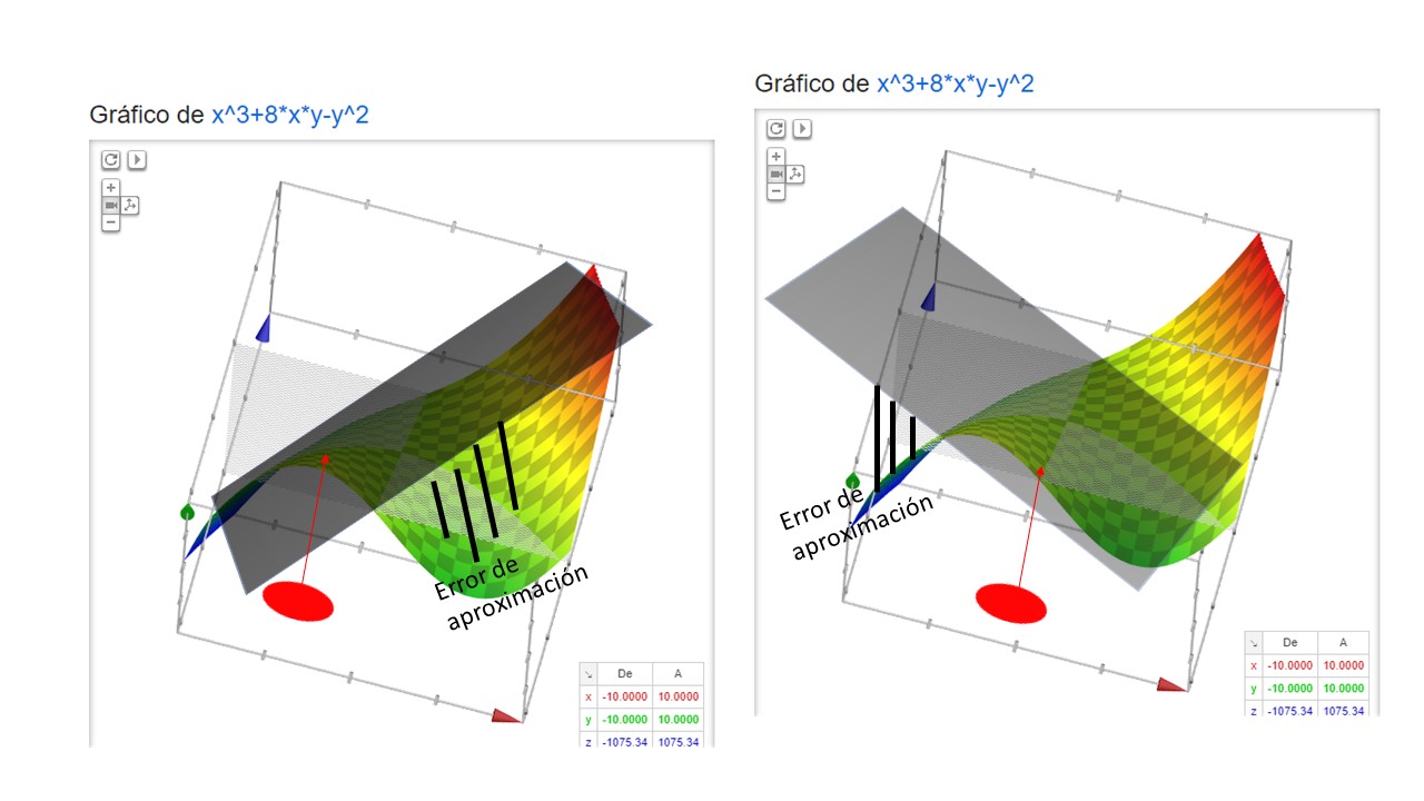
Look at this function: \(f(x,y)=x^{3}+8xy-y^{2}\). Its partial derivatives \(f'_{x}=3x^{2}+8y\) and \(f_{y}'=8x-2y\) as you see, exist (they are polynomials), and are continuous for all values of \(x,y\).

This implies that the function is differentiable at that point. As you can see, in FIG4, when drawing a plane tangent by a point any of these smooth functions, in an environment (delimited by the red ball), the approximation using a plane is good enough.

However, and analogous to what we have already seen in one dimension, there are functions with peaks whose partial derivatives exist but which do not satisfy the sufficient condition of differentiability. If you draw them, you can immediately see that there are points where the function it could not be approached by plans since these would not be unique.

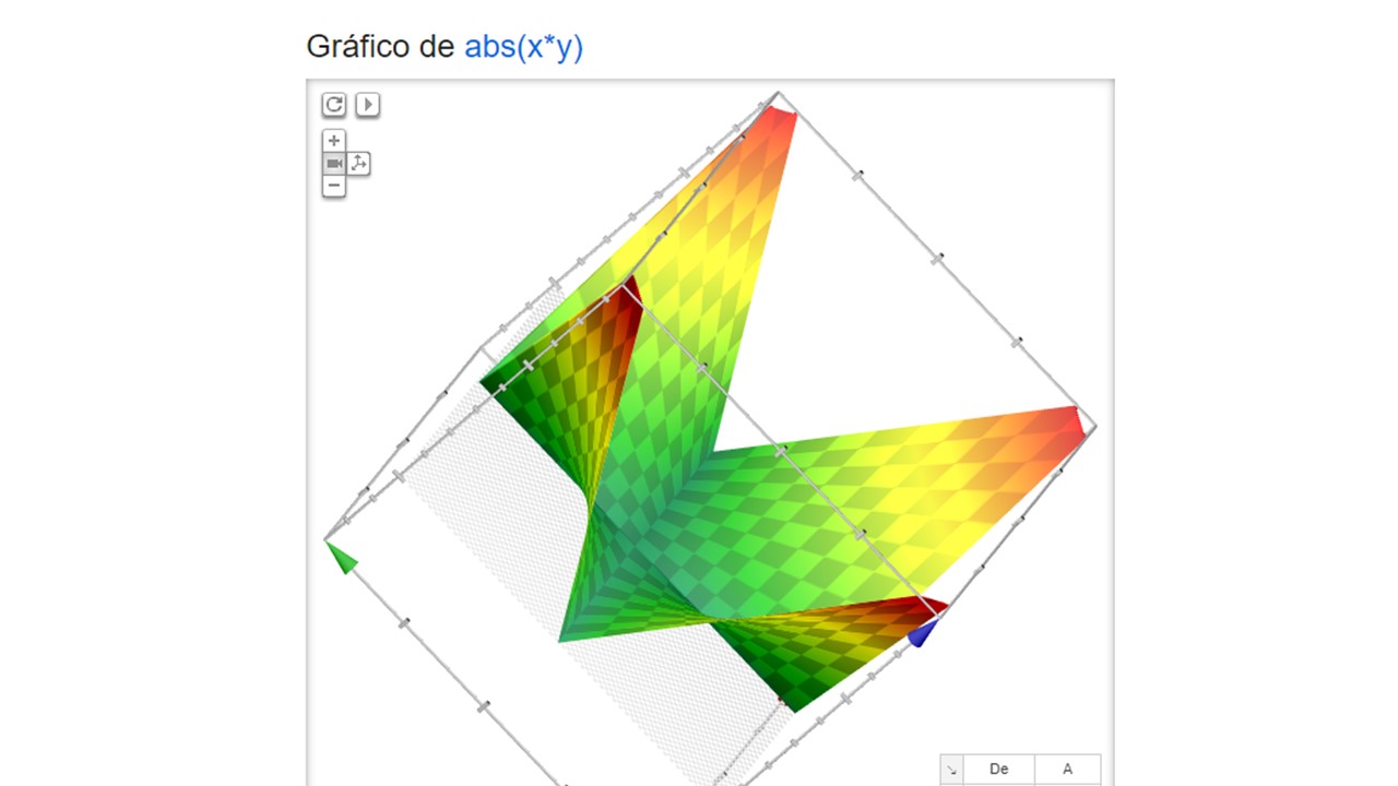
FIG4 Typical function that looks like a crumpled paper. Not differentiable at several points, even if it is continuous.

In this course we will usually work with differentiable functions. If they are differentiable, we say that \(f\in C^{1}\left[(x_{0},y_{0})\right]\) that is, \(f\) is a class 1 function in the point environment \(x_{0}.y_{0}.\) Being a class 1 function implies that sus first partial derivatives exist and are continuas in the environment of that point, this is, meets the sufficient condition of differentiability.

Exercise 2 Let \(g(x,y)=2xy^{\frac{1}{2}}+x\). Say if the following statements:

1. The function \(g(x,y)\) is differentiable at point \((2,4)\)

2. For points \((x,y)\) close to point \((2,4)\) \(g(x,y)\approx5x+y-4\) is met

Exercise 3

Let \(\Pi(r,w)=100\frac{r+w}{rw}\) be the benefit function of a company where \(r\) is the price of capital and \(w\) is the price of labor. It is requested: a) Calculates the gradient vector of the profit function at the point \((r_{0},w_{0})=(2,1)\) and economically interprets the sign of each of the partial derivatives. b) Calculate the Hessian matrix of the given function at the point \((r_{0},w_{0})=(2,1).\) c) Using the differential, calculate the approximate value of \(\Pi(1.99,1.01).\)

Class 9: Gradient properties and use of the Hessian matrix

Let’s try to understand the interesting properties of the gradient, and very useful in optimization, with an example. Let’s look at a simple function:

\[ f(x,y)=ln(4x-y) \]

Suppose we are at the starting point \(x_{0}.y_{0}=(1.3)\). Let’s go to calculate the vector gradiente of the function:

\[ \nabla f(x,y)=\left[\frac{4}{4x-y},\frac{-1}{4x-y}\right] \]

that, evaluated at point \((1,3)\),

\[ \nabla f(x_{0},y_{0})=\left[4,-1\right] \]

Do you remember what information a vector gave us? In this case, having two coordinates, it is marking us in which direction we Move. For example, the vector (4,-1) tells us to always walk 4 steps in the direction of the \(x\) axis (i.e. right) and minus 1 step (i.e. towards abao) in the direction of \(y\) axis. If we draw it, we are going in this direction:

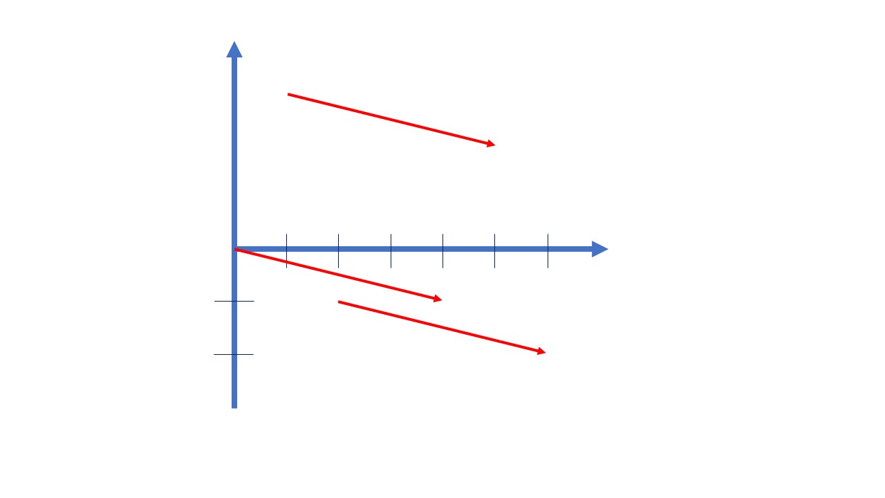
FIG5. The same vector in \(\mathbb{R}^{2}\).

Note that vectors mark the same direction, it doesn’t matter if we start of (0.0). That is, where you start it does not matter, which is the same as say that the point of application of the vector is not important. All these vectors are, in short, the (4,-1).

Well, we have already caught the idea of what a vector is for us (at least, for us). Now let’s go for the next argument. Paints the contour lines of the example function. To do this:

\[ C=ln(4x-y)\Rightarrow e^{C}=4x-y \]

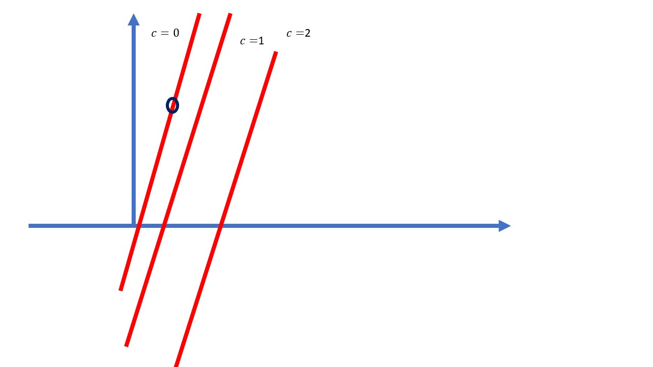
FIG6. the contour lines for different values of c.

As you can see in FIG2, the function grows as we go in a southeasterly direction. Herself can you improve this description?. Now we ask ourselves which of these arrows (yes, yes, vectors) is the one that allows you to move towards the next valor mayor of the feature faster? Check out these Candidates. Which arrow (vector) do you think is the best?

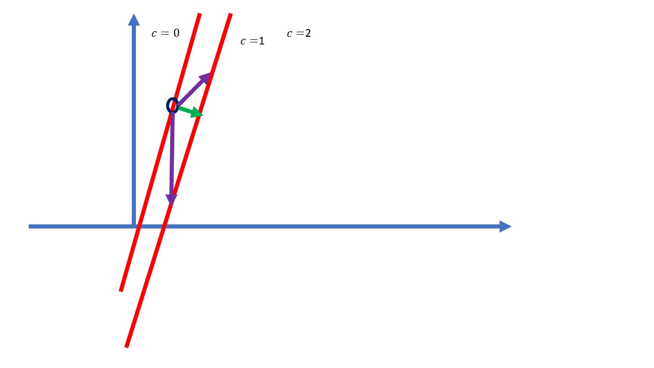
FIG7. The green one!

you will agree with me that the best candidate is the green one. That is the fastest way we find to advance to the next point of the function. Well, look, that vector is proportional to another that we have already drawn before:

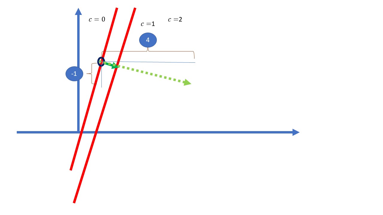
FIG8. Which vector is proportional?

From the gradient! Indeed. In fact, this allows us to state a property (which we do not prove) on the gradient:

The gradient marks the direction of maximum growth/decrease of the function

What is it to look for the direction of maximum growth/decrease of the function?

We need, in this case, to find the displacement vector \((\Delta x,\Delta y)\). That allows me to grow/decrease as fast from a given point \(x_0.y_0\).

We already know that the change in function can be written, so approximate as:

\[ \triangle f\approx\frac{\partial f(x_{0},y_{0})}{\partial x}\triangle x+\frac{\partial f(x_{0},y_{0})}{\partial y}\triangle y \]

So, we see that:

1. The direction of maximum growth is one in which the angle between the gradient and the increment vector is null (i.e. they are the same vector). This means that \(\triangle x,\triangle y\) they must move proportional to the gradient vector.

2. The direction of greatest decrease is the counter (that is, forming 180 degrees with respect to the contour line)

3. There are directions in which it does not vary: if the increment vector is perpendicular to the gradient vector.

Exercise 4 Consider the function \(B(p,Q)=(p-3)Q\). Draws the contour of the function containing the point \((7,8)\). What is the relationship between the contour line and the gradient vector of \(B\) at the point \((7,8)\)? What does this gradient indicate?

Exercise 5

Let be \(f(x,y)=1+x-2y+0.5x^2+3y^2-2xy\), what relationship must satisfy the variations \((\Delta x, \Delta y)\) of the variables so that starting from the point \((0,1)\) the function is increased as quickly as possible?

Exercise 5 Let \(\Pi(r,w)=100\frac{r+w}{rw}\) be the profit function of a company (where \(r\) is the price of capital and \(w\) is the salary) 1) Calculate the gradient vector of the benefit function at the point (2,1) 2) Get the plane tangent to the feature at that point and draw the feature and plane. In what environment does the approach seem acceptable? 3) In what proportion should the price of capital and wages be increased in order for profit to grow as quickly as possible?

Use of Hessian to characterize convexity and concavity of functions

On the other hand, the Hessian matrix will help us characterize a function of two variables \(f(x,y)\) according to their convexity/concavity.

• Convex function: we will say that a function \(f(x,y)\) is convex if the element (1,1) of the Hessian matrix is greater than or equal to zero and the determinant of the Hessian is greater than or equal to zero for all \((x,y)\in\mathbb{R}^2\)

Example: we analyze the function \(f(x,y)=x^2+y^2\). If you draw it in Geogebra you will see that it is a convex function. Sure, the Hessian turns out to be \[Hf(x,y) = \begin{bmatrix}2 & 0\\ 0 & 2 \end{bmatrix}\]

From this matrix, where the element (1,1) is positive and the determinant as well, it is said to be POSITIVE DEFINITE

• Concave function: we will say that a function \(f(x,y)\) is concave if the element (1,1) of the Hessian matrix is less than or equal to zero and the determinant of the Hessian is greater than or equal to zero for all \((x,y)\in\mathbb{R}^2\)

Example: we analyze the function \(f(x,y)=-x^2-y^2\). If you draw it in Geogebra you will see that it is a convex function. Sure, the Hessian turns out to be \[Hf(x,y) = \begin{bmatrix}-2 & 0\\ 0 & -2 \end{bmatrix}\] and complies with the above.

From this matrix, where the element (1,1) is negative and the determinant as well, it is said to be NEGATIVE DEFINITE

• Neither concave nor convex: If the determinant of hessian is less than zero, regardless of what the element is worth (1,1)

Example: the function \(f(x,y)=x^2-y^2\). If you draw it in Geogebra, you will see that it has the shape of a “horse on-board chair.” The Hessian turns out to be \[Hf(x,y) = \begin{bmatrix}2 & 0\\ 0 & -2 \end{bmatrix}\] with negative determinant.

From this matrix, where the determinant element is negative, it is said to be INDEFINITE

Exercise Analyzes the convexity/concavity of the following functions by drawing the function in Geogebra and analyzing its Hessian 1) \(f(x,y)=3x^2+8y^2\) 2) \(f(x,y)=x+2y\) 3) \(f(x,y)=xy\) 4) \(f(x,y)=x^4+y^4\) 5) \(f(x,y)=x^2y\) 6) \(f(x,y)=x^2y^2\)

As you have seen, these conditions are “sufficient” that means that there are functions that do not satisfy them and yet are concave/convex. Of course, if they satisfy them, they are automatically.

We will need this in the function optimization block.