BLOCK 3: Introduction to Optimization

Class 1 (Magistral): Optimization in a variable (I)

An optimization problem in a variable can be posed as a maximization or minimization problem as follows

\[ \max_{x\in D}f(x) \]

\[ \min_{x\in D}f(x) \]

that is, what we want to write is

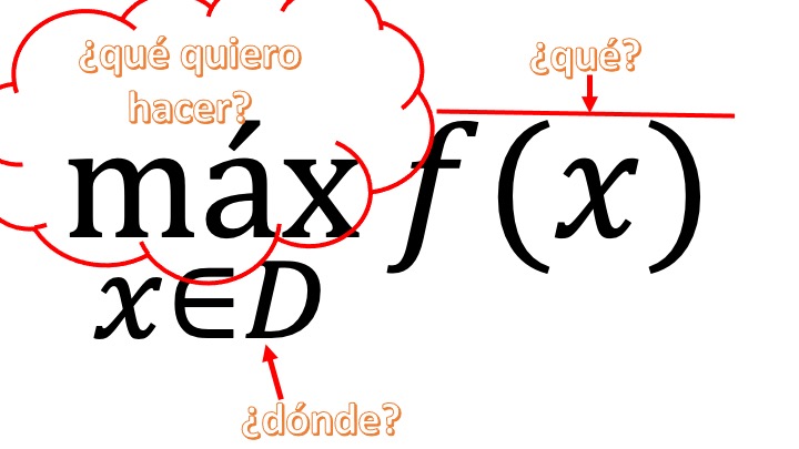
FIG 1 A general problem

• first: what do I want to do: maximize or minimize? If I don’t know, I can put “\(opt\)” instead (which will mean: I want to “optimize”)
• second: what do I want to optimize? generally, a function. in this class also functions of a variable
• third: where do I look for the \(x\) values that optimize my function? Well, as seems logical in the domain of function. When this is the case, and the domain is \(\mathbb{R}\), we will say that the optimization is “free.” If we look for the optimal in an interval, (for example, the domain is \(3<x<5\)) then the optimization with which we will work will be restingida

1.3.2 Free optimization for functions \(\mathbb{R}\rightarrow\mathbb{R}\)

In the search for the maximums or minimums that we have previously enunciated, we can find different possibilities. We analyzed it for minimums but it would be the same for maximums (changing the orientation of inequalities). Watch this FIG2

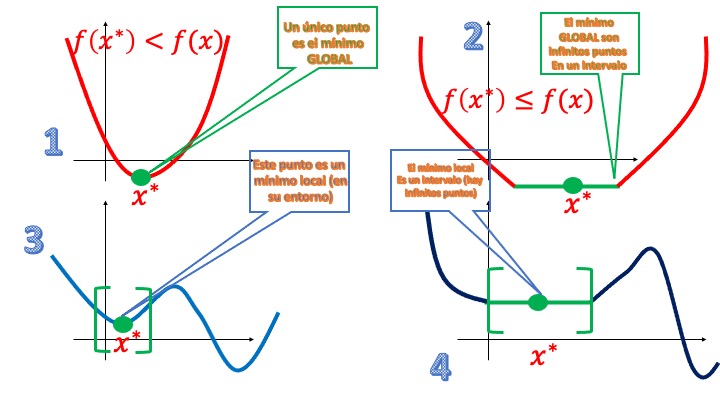
FIG 2 Different types of minimums

1: A point \(x^*\) is a strict global minimum of \(f\) if \(f(x^*)<f(x)\) for all \(x\in\mathbb{R}\). Look closely: of all the possible values of \(x\) on the real line there is only one that is the one that provides the lowest value of the function

2: A point \(x^*\) is a global minimum of \(f\) if \(f(x^*)\leq f(x)\) for all \(x\in\mathbb{R}\). Look closely: of all the possible values of \(x\) on the real line there is an interval of them (all equal to \(x^*\)) which provide the lowest value of the function*

3: A point \(x^*\) is a strict local minimum of \(f\) if \(f(x^*)<f(x)\) for all \(x\in B(x^*)\), where \(B(x^*)\) is a point environment. Look closely: in the environment of \(x^*\), this turns out to be the one that gives the lowest value of the function. But it is local since there is another minimum (local) that gives an even lower value of the function*

4: A point \(x^*\) is a local minimum of \(f\) if \(f(x^*)\leq f(x)\) for all \(x\in B(x^*)\), where \(B(x^*)\) is an environment of the point. Look closely: in the environment of the interval that contains \(x^*\), that interval turns out to be the one that gives the lowest value of the function. But it is local since there is another minimum (local) that gives an even lower value of the function*

We will try to discover, intuitively, all the conditions we need to make sure what situation we are in. We will need to recover, of course, something that we already saw in the applications of the derivatives in functions of a variable

Critical Point or first-order necessary condition

A \(f\) function will have a critical point \(x^*\in \mathbb{R}\) if \(f'(x^*)=0\) or \(f'(x^*)\) does not exist.

That is, the points we seek must satisfy that condition (that’s why we say it’s NECESSARY). Then we will have to classify them.

Example 1 Look for the critical points of \(f(x)=2-x^4-2x^2\) and \(g(x)=e^{x^4}\)

• In the first case, \(f'(x)=-4x^3-4x\). Equaling zero, we have \(4x^3+4x=0\), from which we get the only critical point, which is \(x^*=0\).
• In the second case, \(g'(x)=e^{x^4}(4x^3)\) If we equal this derivative to zero, again we obtain that the only critical point is \(x^*=0\)

Now, what kind of hotspots are they? Are they maximums, minimums, turning points? To do this, we must learn what we will know as a second-order condition.

Second-order necessary condition: local optimums

a point \(x^*\in \mathbb{R}\) that satisfies \(f'(x^*)=0\)

• Local minimum if \(f''(x^*)\geq 0\)
• Local maximum if \(f''(x^*)\leq 0\)

This condition is known as THE SECOND-ORDER NECESSARY CONDITION of local optimum. When \(f''(x^*)= 0\) we can be at minimum, maximum or turning point, as you know.

The necessary second-order condition allows us to classify critical points. For now, as we only take into account the value of the critical point, the analysis is carried out in an environment of the point, in such a way that we can only do a local analysis (hence we can not yet say anything about the globality)

Example 2 Let us think, then, about the functions of Example 1.

• We get the second derivative \(f''(x)=-12x^2-4\). Particularizing at the critical point $f’’(0)=-$4. Therefore, we know that it is a local maximum
• In the second case, \(g''(x)=e^{x^4}(4x^3)^2+12x^2e^{x^4}\) evaluating at the critical point \(f''(0)=0\) so that it meets the condition of both maximum, local minimum or inflection point.

Note These conditions can be made “necessary and sufficient” by simply restricting the local maximum condition if $f’’(x^)< $0 or local minimum if $f’’(x^)>$0.

If we want to analyze the possible globality of the critical point, then we must use an important theorem.

Local-Global

A function \(f\), differentiable:

-convex across its domain: local minimums are global -concave across its domain: local highs are global

Remember that a function is convex throughout its domain if, for all \(x\in D\) the second derivative is greater than or equal to zero and is concave throughout its domain if, for all \(x\in D\) the second derivative is less than or equal to zero.

Applying the local-global theorem to the above functions, we can see

• In the first case, \(f''(x)=-12x^2-4\) is always NEGATIVE, that is, for any \(x\), the second derivative is strictly less than zero. So, we know that the function is strictly concave. By the local-global theorem, the critical point $x^=$0 is automatically global maximum*.
• In the second case, \(g''(x)=e^{x^4}(4x^3)^2+12x^2e^{x^4}\) is always GREATER THAN OR EQUAL TO ZERO It is a convex function and, therefore, the critical point \(x^*=0\) is a global minimum.

These conditions – together with the Local-Global Theorem – will help you make the corresponding decisions. In essence, we use the necessary conditions to discriminate whether a point can be an optimal point, while enough help us classify them (although with limitations, since not meeting a sufficient condition does not assure you anything, although meeting it does). Let’s go with examples

Example 3

Let’s use what we have learned to classify the critical points of \(f(x)=x^3\), \(g(x)=3x^5-5x^3\), \(h(x)=\sqrt(x)+2ln(x)\), \(i(x)=\frac{1}{1+x^2}\)

First derivative	Second	derivative Does Local Global Comply?
\(f'(x)=3x^2\)	\(f''(x)=6x\)	NO
\(g'(x)=15x^4-15x^2\)	\(g''(x)=60x^3-30x\)	NO
\(h'(x)=\frac{-1}{2\sqrt(x)}+\frac{2}{x}\)	\(NA\)	\(NA\)
\(i'(x)=\frac{-2x}{(1+x^2)^2}\)	\(i'(x)=\frac{6x^2-2}{(1+x^2)^3}\)	\(NO\)

Let’s go case by case

• 1. The critical point is only \(x^*=0\). The second derivative, as we see, changes sign according to \(x\), so it does not satisfy the local-global theorem (which would require a single sign for all \(x\)). If you look, \(f''(0)=0\), which could be at least local maximum. Now, since the local-global theorem is not fulfilled, we must think something else: if we look, the second derivative changes sign to the left and right of the critical point. Remember that this characteristic is that of TURNING POINT. It is already classified.

• 2. we have 3 critical points: \(x^*_1=0\), \(x^*_2=1\), \(x^*_3=-1\). As we can see, the local-global theorem does not apply, since the second derivative changes sign according to the value of \(x\) and, therefore, is neither concave nor convex. If we evaluate the second derivative in each of the points (to be able to classify them as local), we will have \(f''(0)=0\) so it can be maximum or minimum or turning point, \(f''(1)=30\), so it is a local minimum and \(f''(-1)=-30\) for or that is a local maximum. We cannot know if they are global, since the local-global theorem is not satisfied. One idea we can do is to see its graph. If you don’t have it available, you can think about whether the feature can get best and worst maximums and minimums. Take the calculator: we know that in \(x =1\) we have a minimum (local). There the function is worth \(g(1)=-2\). If it were a global minimum, we would be unable to find a value for \(g\) less than \(-2\) for any other \(x\). But look: \(g=3x^5-5x^3\). You can find, surely, values for \(x\) that make \(g\) less than \(-2\). For example, if $x=-$3, $g(-3)=-$594. That’s because, if you look, if \(x\rightarrow -\infty\), then \(g\rightarrow -\infty\). You will see that the same thing happens with \(x=-1\) is a local maximum. $x=$0 is a turning point, as the second derivative changes sign to the right and left of \(x=0\). This has cost, since if the Local-Global Theorem is not fulfilled, everything is more tedious.

• 3), as you can see, the first derivative does not exist when \(x^*=0\): but \(x=0\) is not a point of the domain, so this function has no critical point: it is always increasing.

• 4. has a single critical point: \(x^*=0\). The local-global theorem is not fulfilled because the second derivative changes with the value of \(x\). However, $i’’(0)=-$2, so it’s a strict local maximum. To know if it is global, we must think if there are values of \(x\) that make this function can take values greater than \(i(0)=1\). To do this, you must think about the function \(i=\frac{1}{1+x^2}\). If you notice, the higher/lower \(x\), this function is approaching zero, so the maximum we have found is global.

Domain of the objective function defined in a closed interval: we do not need the second derivative

In the case in which it is defined that the domain of the function in which it is interesting to look for the optimum is in a closed interval, the following points must be analyzed:

\(x\in[a,b]\)

• the points where the derivative of the function cancels or does not exist
• the ends of the interval

When the domain is defined in a closed and bounded interval, we say that it is defined in a compact set. Weierstrass’s theorem states that, then, if the objective function is continuous, the problem will have global minimum and maximum. To know what they are you just have to make a table with the values of the function of the previous points.

Let’s look at an example:

Example 1 Find the optimals of the function \(f(x)=x^{2/3}(5-2x)\) if \(x\in[-1,2]\)

solution Since the function is defined in a closed interval, we know that we must analyze the value that the function takes at the ends of the interval. In addition, we must obtain the critical points of this. We have to

\[ f'(x)=\frac{10}{3}x^{-1/3}(1-x) \]

Where we can see that, if \(x^*=1\), the derivative is canceled out and if \(x=0\) the derivative does not exist (since the cube root is in the denominator). So, since the range of the \(x\) is closed, we can make a table of values to know which \(x\) provides the highest value to the function and the lowest

Value \(x^*\)	\(f(x^*)\)	What kind of point is it?
$x=-$1	\(7\)	Maximum GLOBAL
$x=$0	\(0\)	Global Minimum
\(x=1\)	\(3\)
\(x=2\)	\(1.59\)

Domain of the target function defined in an open interval

If the function is defined on an open interval, then it does not take values at the ends of the interval, so they are no longer points that we should contemplate (although what happens to the function when it approaches those points)

\(x\in(a,b)\)

• the points where the derivative of the function cancels or does not exist
• The limit of the function when approaching \(a\) and \(b\)

Now the Weierstrass Theorem no longer applies, since the interval where the \(x\) is defined is not closed. Let’s look at an example:

Example 2 Find the optimals of the function \(f(x)=x^{2/3}(5-2x)\) if \(x\in(-1,2)\)

solution We already know the critical points. Let’s use the second derivative (whenever possible) to characterize them:

\[ f''(x)=\frac{-10}{9}x^{-4/3}(1-x)-\frac{-10}{3}x^{-1/3} \]

Where we can see that, if \(x^*=1\), the second derivative is negative (so it is a local maximum) and in \(x=0\), obviously, the second derivative does not exist. However, the first derivative is negative when \(x<0\) and positive when \(x>0\). So, we know it’s a local minimum. We study these points, as well as what happens to the function if it approaches the extremes.

Value \(x^*\)	\(f(x^*)\)	What kind of point is it?
$x-$1	$f(x)$7	NOTHING
$x=$0	\(0\)	Global minimum
$x=$1	\(3\)	Local maximum
$x=$2	$f(x)$1.59	NOTHING

**we see that $x=$1 is a local maximum (since when we approach $x=-$1, the function is greater than \(3\)). However, in this range \(x=0\) becomes the GLOBAL minimum.

How to work reasonably?

We recommend:

1. First look for the critical points (first-order necessary condition)

2. Analyzes the interval where the variable is defined (is it closed?) If it is closed, use the Weierstrass theorem: you do not need to analyze the second derivatives, you can directly find the GLOBAL maximum and minimum (s).

3. If the interval is not closed, think if you satisfy, by the second derivative, the local-global theorem (if so, decide if it is a problem of global maximization or minimization)

4. Then classify each critical point with the second derivative (second-order necessary/sufficient conditions)

5. As you can see, this is not just following a recipe: you also need some ART.

This is summarized in two videos:

• In this the necessary and sufficient conditions of optimal are defined

• This is a review of how to approach an optimization problem

Project: the warehouse An optician buys 600 sunglasses of one model a year. The cost of each shipment is 50 euros. The cost of storage is 1 euro per pair per year. Each pair costs, to the seller, 20 euros. Suppose they are sold at a steady $a rate over time (days) and the shipment arrives when stocks run out of the previous shipment. How many glasses do you have to order per batch to minimize the cost?

• We will call \(x\) to the stored units and to \(t\) to the time in days. On average, there are $x/$2 glasses in the warehouse. Why? Because inventory always starts at \(x\) glasses and ends at \(0\). The average is $x/$2.

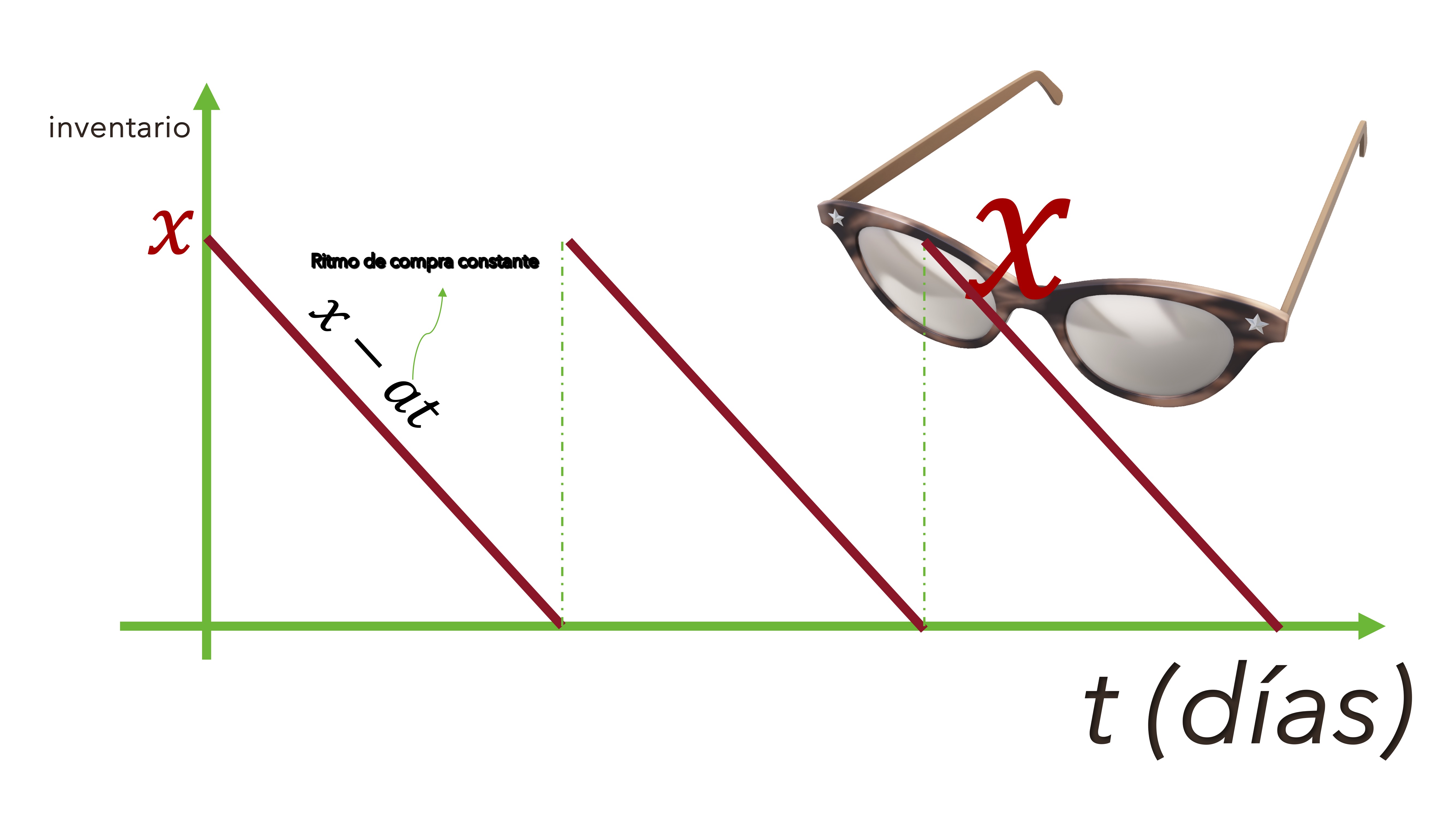
FIG 3 Warehouse diagram

• The average cost of storing in each cycle will be \(C_{A}=1 euro \times \frac{x}{2}\), \(C_{A}=\frac{x}{2}\).

• How much do shipments cost? are 50 euros for the total shipments. That total will be 600 glasses among the number of glasses per shipment. That is, \(C_{E}=50\times \frac{600}{x}\)

• What is the total cost of the glasses? $C_{G}=20=$12000 is the fixed cost of the entrepreneur.

The sum of all these costs provides us with the total:

\[ C_{T}=\frac{x}{2}+\frac{30000}{x}+12000 \] realize, on the other hand, that the cost must be minimized by taking into account that \(x\in (0,600]\). The interval is open on the left and closed on the right.

*How do we solve the problem using the guide?

How to work reasonably?

We recommend:

1. First look for the critical points. If we make the first derivative, we have to \(f'(x)=0.5-\frac{30000}{x^2}\). This does not exist if \(x=0\) but that point is not in the domain. On the other hand, this is canceled (i.e. \(0.5-\frac{30000}{x^2}=0\)) if $x=$245 or $x=-$245. We are left with $x=$245, which is the one in the domain.

2. Analyzes the interval where the variable is defined (is it closed?) If it is closed, it uses the Weierstrass theorem. The interval, as we have said, is not closed by the left, so it does not satisfy this theorem.

3. If the interval is not closed, think if you satisfy, by the second derivative, the local-global theorem The second derivative is \(f''(x)=\frac{600}{x^3}\). In the domain of \(x\) this derivative will always be positive. Then, this function is convex in that span and the local minimum automatically becomes global.

Another way to proceed is by analyzing the critical points as local and then thinking about their globality. In that case, you don’t need to analyze the convexity/concavity of the objective function: it’s somewhat more laborious. You can analyze the value of the target function at the critical points to later see how much the target function is worth in $x=$600, which is where it is closed and what value the target function is close to if \(x\) approaches zero (it can never be worth \(0\)), In that case, it is easy to see that the cost is going to infinity and that when $x=$600 the cost is higher than at the critical point. That is why we say that it is a global minimum.

We already know that the optimal policy is to choose $x= $ 245 with a cost of 12245 euros.

Class 2 (master): Free optimization in functions \(\mathbb{R^2}\rightarrow\mathbb{R}\)

Problem statement

Our goal is, now, to look for the optimal in a function of two unrestricted variables in those variables. We will write the problem like:

\[ \underset{(x,y)\in\mathbb{R}^{2}}{opt}f(x,y) \]

If the objective function is differentiable (has partial derivatives) first and second continuous), we can use the tools of differential calculus learned in BLOCK 2 to be able to efficiently solve the problem.

FIRST ORDER NECESSARY Conditions

What are they for?

• They allow us to find critical points that may be: maximum, minimum or chair points.

• When necessary: exclude as candidates for optimal those points that can never be, but will include points that later cannot be will be optimal

• They are based on the information provided by the gradient.

Si \(f(x,y)\) is differentiable and the point \((x^{*},y^{*})\) is an optimal, verify that
- \(\nabla f(x^*,y^*)=(0,0)\)

This condition is known as THE FIRST ORDER NECESSARY CONDITION of local optimum. It is analogous to the case with a variable.

This condition (which, for short, is usually denoted as CPO), will allow us to obtain a set of critical points that will be the optimal candidates of the problem. We will have three possible points: maximums, minimums or chair points. As you can see in FIG 1, it is easy to visually characterize these points:

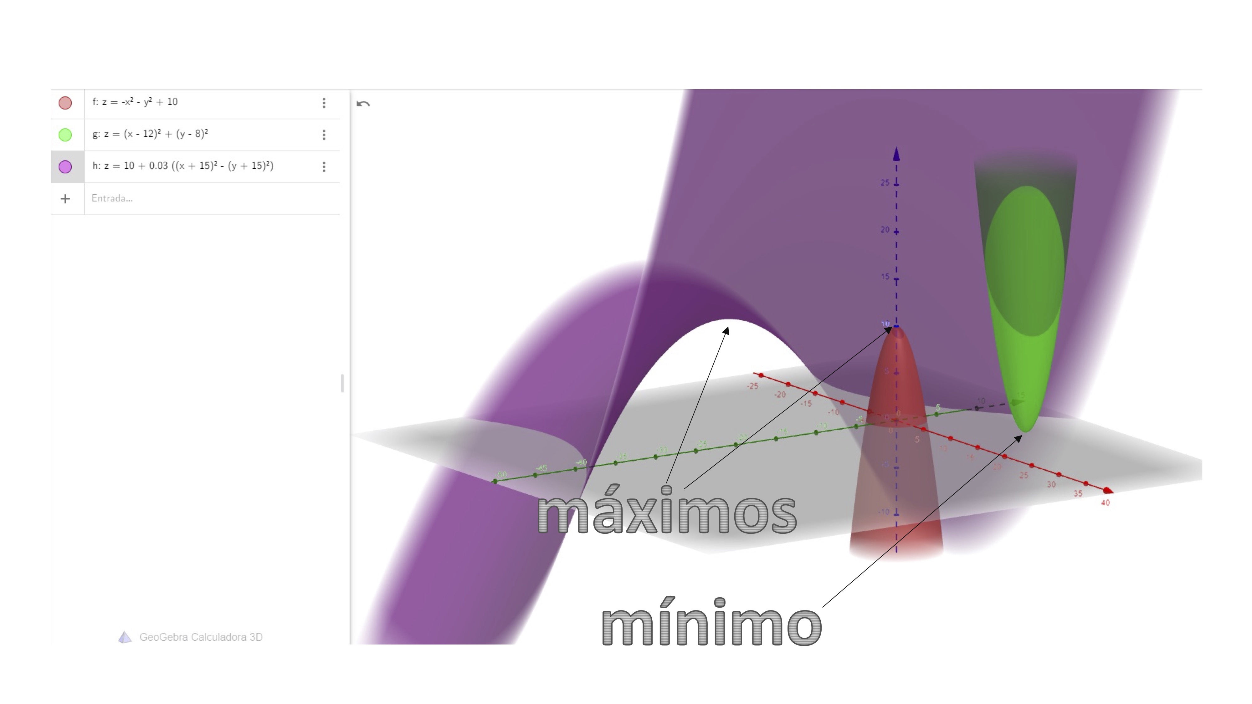
FIG 1 The red function has a maximum and the green one a minimum… The abode seems to have a maximum (local), doesn’t it?

But something happens with the purple function. Let’s rotate the drawing, as you will see in FIG2:

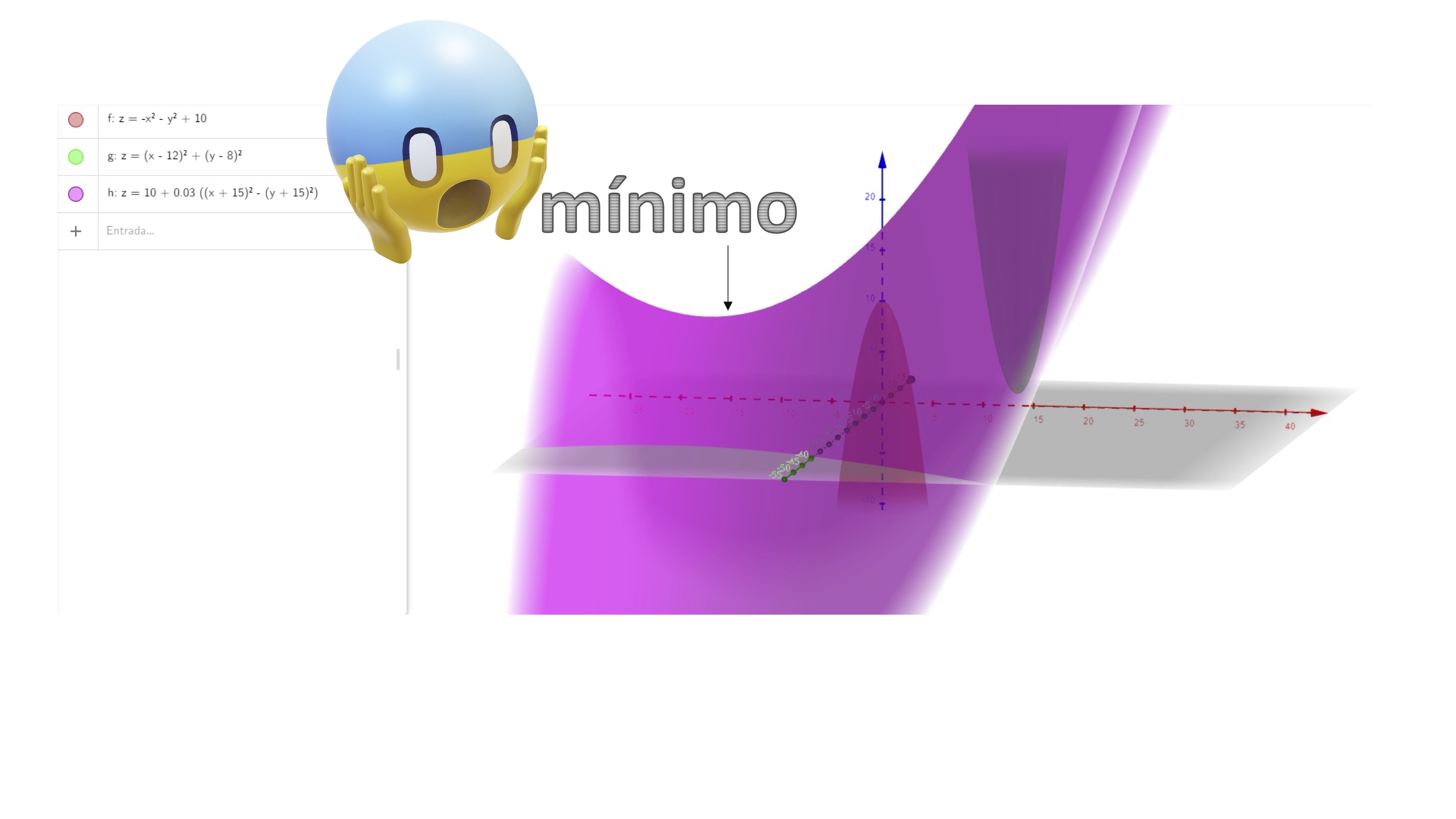
FIG 2 Look, if you rotate it, then it seems a local minimum, arggg!

Ah, it seems that the purple function has a chair point.

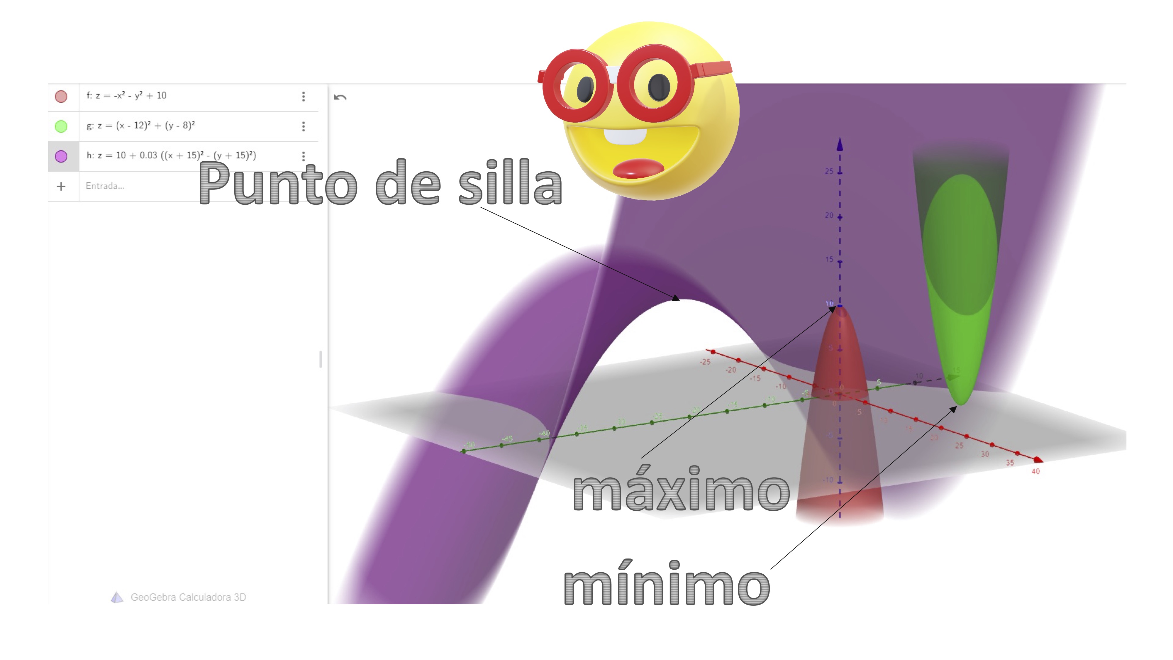
FIG 3 It’s a chair point!

That is, we define as:

• Local maximum: in an environment, it is the point (or set of points) that provide the highest value to the function

• Local minimum: In an environment, it is the point (or set of points) that provide the least value to the function

• Chair point: in an environment, it is the point (or set of points) that provide less value to the function (in a possible direction) and higher value to the function (in another possible direction).

Exercise resolved

Calculate the minimums, maximums (local) and chair points of the function of two variables:

\[ f(x,y)=x^{3}+y^{3}+2x^{2}+4y^{2}+6 \]

So, we apply:

• Necessary conditions of the first order: \[ \nabla f(x,y)=(0,0), \]

that is, we get the system:

\[ \begin{cases} 3x^{2}+4x=0\\ 3y^{2}+8y=0 \end{cases} \]

We solve it:

\[ \begin{cases} x(3x+4)=0\Rightarrow x=0,x=\frac{-4}{3}\\ y(3y+8)=0\Rightarrow y=0,y=\frac{-8}{3} \end{cases} \]

Where the solution is the following four points

\[ A(0,0),B\left(-\frac{4}{3},0\right),C\left(0,-\frac{8}{3}\right),D\left(-\frac{4}{3},-\frac{8}{3}\right) \]

How do we rank these points? We need more condiciones

NECESSARY conditions of the second order

What will we use them for?

• They serve to characterize (i.e., label) critical points as “local highs,” “local lows,” or “chair points,” without saying anything about globality.

• It does not identify strict minimums/maximums.

• Again, being optimal necessary conditions, there will be points that satisfy them and that are chair points (that is, NOTHING for the purpose of optimizing).

But the novelty is that: we now use the Hessian information (i.e. the second derivatives)

Si \(f(x,y)\) is differentiable and has, in addition, continuous second partial derivatives in \(\mathbb{R}^{2}\), it is verified that:
- \(\nabla f(x^*,y^*)=(0,0)\)

Type	First Order	Second Order
maximum local	\(\nabla f(x^*,y^*)=(0,0)\)	\(Hf(x^*,y^*)\) semi-defined negative
local minimum	\(\nabla f(x^*,y^*)=(0,0)\)	\(Hf(x^*,y^*)\) semi-defined positive
	chair point \(\nabla f(x^*,y^*)=(0,0)\)	\(Hf(x^*,y^*)\) Indefinite

And we define,

Una matriz \(2\times2\) \(A=\left[\begin{array}{cc} a_{11} & a_{12}\\ a_{21} & a_{22} \end{array}\right]\)

is semi-defined negative if \(a_{11}\leq0\) and \(\left| A\right|\geq0\). It is semi-defined positive if \(a_{11}\geq0\) and \(\left| A\right|\geq0\). It is indefinite if \(\left| A\right|=0.\) In this case, there is also another comfortable way to classify the points according to the “eigenvalues” of the matrix. Eigenvalues, \(\lambda_{1},\lambda_{2}\) solve this equation:

\[ \left|\left[\begin{array}{cc} a_{11}-\lambda & a_{12}\\ a_{21} & a_{22}-\lambda \end{array}\right]\right|=0\Rightarrow\lambda^{2}-(a_{11}+a_{22})\lambda+\left| A\right|=0 \]

and, through the criterion of self-values, we can say that

Type	First Order	Second Order
maximum local	\(\nabla f(x^*,y^*)=(0,0)\)	\(\lambda_{1},\lambda_{2}\geq0\)
local minimum	\(\nabla f(x^*,y^*)=(0,0)\)	\(\lambda_{1},\lambda_{2}\leq0\)
	chair point \(\nabla f(x^*,y^*)=(0,0)\)	\(\lambda_{1}\neq0\),\(\lambda_{2}\neq0\) and of different sign.

If \(\lambda_{1}=0\), we are in trouble!: the available information will not allow us to characterize the critical points. There is not always a clear answer. Then, we’ll look at examples.

SUFFICIENT second-order conditions

• They serve to characterize (i.e., label) local optimums, without saying anything about globality.

• The novelty is that it allows to ensure if these are strict.

Si \(f(x,y)\) is differentiable and has, in addition, continuous second partial derivatives in \(\mathbb{R}^{2}\), it is verified that:

Type	First Order	Second Order
maximum local	\(\nabla f(x^*,y^*)=(0,0)\)	\(Hf(x^*,y^*)\) Negative defined
local minimum	\(\nabla f(x^*,y^*)=(0,0)\)	\(Hf(x^*,y^*)\) Positive defined
	chair point \(\nabla f(x^*,y^*)=(0,0)\)	\(Hf(x^*,y^*)\) Indefinite

Caution!, it is a sufficient condition

If a point does not meet it, it does not mean that it cannot be optimal.

Definition:

A matrix \(2\times2\)

\(A=\left[\begin{array}{cc} a_{11} & a_{12}\\ a_{21} & a_{22} \end{array}\right]\)

is defined negative if \(a_{11}<0\) and \(\left| A\right|>0\). It is defined positiva si \(a_{11}>0\) y \(\left| A\right|>0\). Es indefinida si \(\left| A\right|=0.\)

In this case, there is also another comfortable way to rank the points. attending to the “eigenvalues” of the matrix. Self-values, \(\lambda_{1},\lambda_{2}\) solve this equation: \[ \left|\left[\begin{array}{cc} a_{11}-\lambda & a_{12}\\ a_{21} & a_{22}-\lambda \end{array}\right]\right|=0\Rightarrow\lambda^{2}-(a_{11}+a_{22})\lambda+\left| A\right|=0 \]

Type	First Order	Second Order
maximum local	\(\nabla f(x^*,y^*)=(0,0)\)	\(\lambda_{1},\lambda_{2}>0\)
local minimum	\(\nabla f(x^*,y^*)=(0,0)\)	\(\lambda_{1},\lambda_{2}<0\)
	chair point \(\nabla f(x^*,y^*)=(0,0)\)	\(\lambda_{1}\neq0\),\(\lambda_{2}\neq0\) and of different sign.

Let’s go back to the solved example

From the previous example, with critical points \[ A(0,0),B\left(-\frac{4}{3},0\right),C\left(0,-\frac{8}{3}\right),D\left(-\frac{4}{3},-\frac{8}{3}\right) \],

the second partial derivatives are

\[ \frac{\partial^{2}f}{\partial x^{2}}=6x+4 \]

\[ \frac{\partial^{2}f}{\partial y^{2}}=6y+8 \]

\[ \frac{\partial^{2}f}{\partial x\partial y}=\frac{\partial^{2}f}{\partial y\partial x}=0 \]

which provide us with a Hessian matrix:

\[ Hf(x,y)=\left(\begin{array}{cc} 6x+4 & 0\\ 0 & 6y+8 \end{array}\right) \]

and we are going to analyze it for each point:

Point	Hessiana	Type
\(A(0,0)\)	\(Hf(0,0) = \begin{bmatrix} 4 & 0\\ 0 & 8 \end{bmatrix}\)	Positive defined (strict local minimum)
\(B\left(-\frac{4}{3},0\right)\)	\(Hf(\frac{-4}{3},0)=\begin{bmatrix} -4 & 0\\ 0 & 8 \end{bmatrix}\)	Indefinite & Chair Point
\(C\left(0,-\frac{8}{3}\right)\)	\(Hf(0,\frac{-8}{3})=\begin{bmatrix} 4 & 0\\ 0 & -8 \end{bmatrix}\)	Indefinite & Chair Point
\(D\left(-\frac{4}{3},-\frac{8}{3}\right)\)	\(Hf(\frac{-4}{3},\frac{-8}{3})=\begin{bmatrix} -8 & 0\\ 0 & -8 \end{bmatrix}\)	Negative Set & Strict Local Maximum

Exercise uses the criterion of eigenvalues to classify the matrix.

Global Optimums: The Local-Global Theorem

So far we have only presented conditions of local optimum, already that the above techniques are based on analyzing hessian of the function in the environment of the candidate points. The Local-Global Theorem states:

Global Local Theorem in a Free Optimization Problem in Two Variables

If the objective function \(f(x,y)\) is differentiable y:

-convex, local minimums are global. -concave, local highs are global.

Remember How do we know if a function is convex or concave? We must analyze hessian. If it is positive semidefinite for every point, then the function will be convex and if it is negative semidefinite it will be concave. Furthermore, if it is positive definite, then it is strictly convex implying that there is only one global minimum and vice versa if it is negative definite.

Example : Is \(f(x,y)=x^{2}+y^{2}\) convex?

In the drawing it is clearly seen, but let’s see it analytically \[ \Delta f(x,y)=\left[2x,2y\right] \]

What is Hessian to be? \[ Hf(x,y)=\left[\begin{array}{cc} 2 & 0\\ 0 & 2 \end{array}\right] \]

as you can see, it is Positive Definite for any value of \((x,y)\). So, it is strictly convex and-therefore- the candidate for local minimum we know will be, automatically, global.

Example where everything fails ranks the \((0.0)\) point into the following minimization problem

\[ \min f(x,y)=x^{3}-3xy^{2} \]

First we must ensure that it is a critical point, that is, that it meets the necessary first-order condion

\[ \nabla f(x,y)=\left[3x^{2}-3y^{2},-6xy\right] \]

as we see, \(\nabla f(0,0)=\left[3\times0^{2}-3\times0^{2},6\times0\times0\right]=[0,0]:\) it fulfils the necessary condition of the first order. Let’s get the Hessian \[ Hf(x,y)=\left[\begin{array}{cc} 6x & -6y\\ -6y & 6x \end{array}\right] \]

Evaluating the Hessian at (0,0), we have \[ Hf(0,0)=\left[\begin{array}{cc} 0 & 0\\ 0 & 0 \end{array}\right] \]

As we can see, with regard to the necessary conditions of the second order, we do not know if it is maximum, minimum or chair point. The test is inconclusive.

Moreover, we do not satisfy the global local theorem. Here we will have to utilizar some imaginación and we will have to analyze what happens in the environment of the critical point (0,0)

\[ f(x,0)=x^{3} \]

as we see, if \(x>0\), the function (in the environment of \((0,0)\)) takes positive values and if \(x<0\), negative values. That is, if we approach from the left, on the axis of the \(x\) we are facing a maximum and, if we approach from the right, before a minimum. Then it must be a chair point.

Again, you can check this content in two videos

• In this the necessary and sufficient conditions of optimal are defined

• This is a review of how to approach an optimization problem

Class 3 OPTIMIZATION WEEK: Introduction to feature-restricted optimization \(\mathbb{R^2}\rightarrow\mathbb{R}\)

Let’s solve, graphically, the following problem:

\[ \min_{x,y}x^{2}+y^{2} \]

subject to:

\[ x+2y=10 \]

As you can see, we incorporate a restriction: the \((x,y)\) points that minimize the objective function must satisfy the equation $x+2y=$10. Let’s go to try to solve it graphically, following some concrete steps.

• Sketch the contour lines of the target function

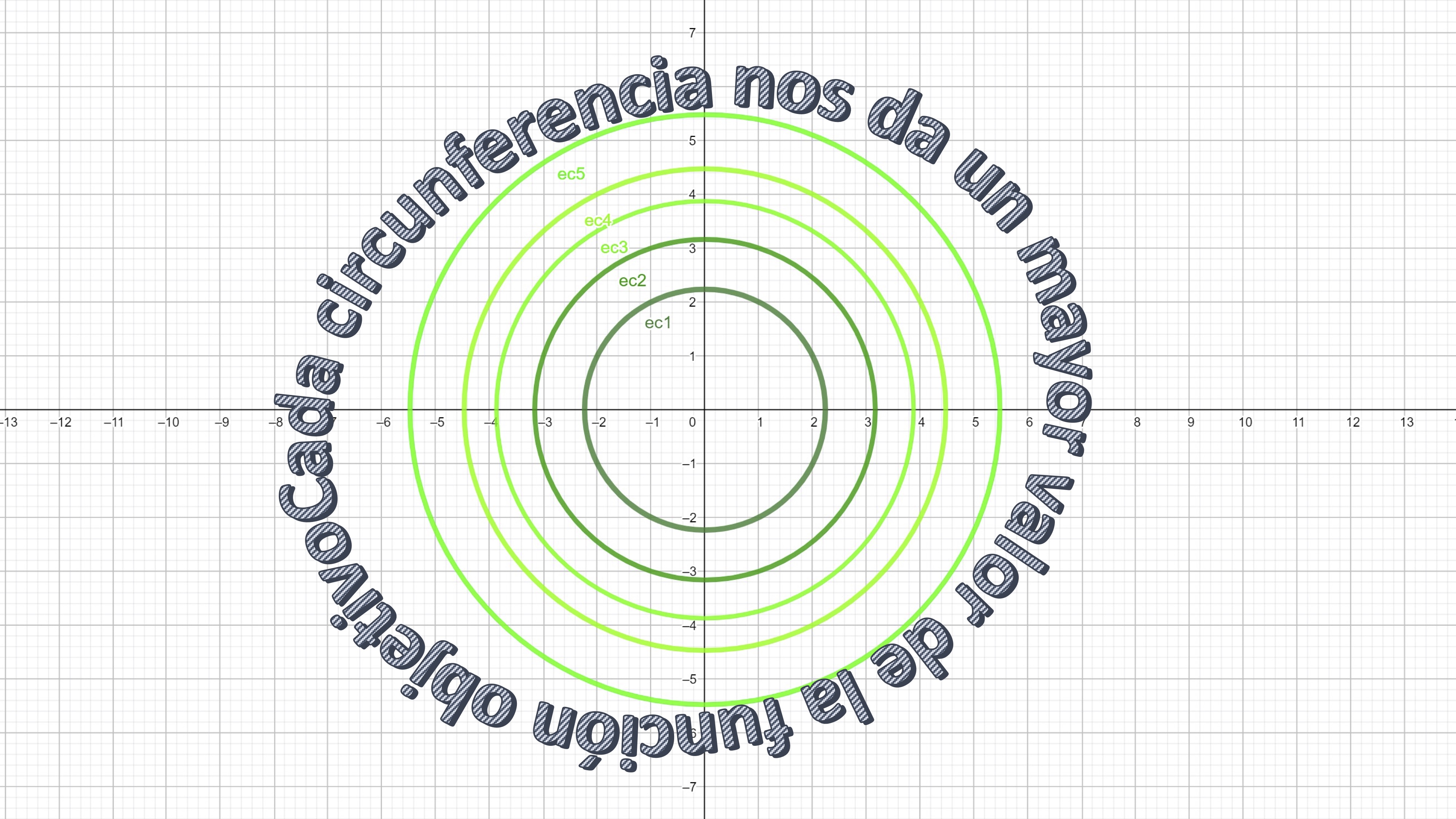
FIG 1 You already know these contour lines, don’t you?

• Includes restriction \((x+2y=10)\) on the same chart

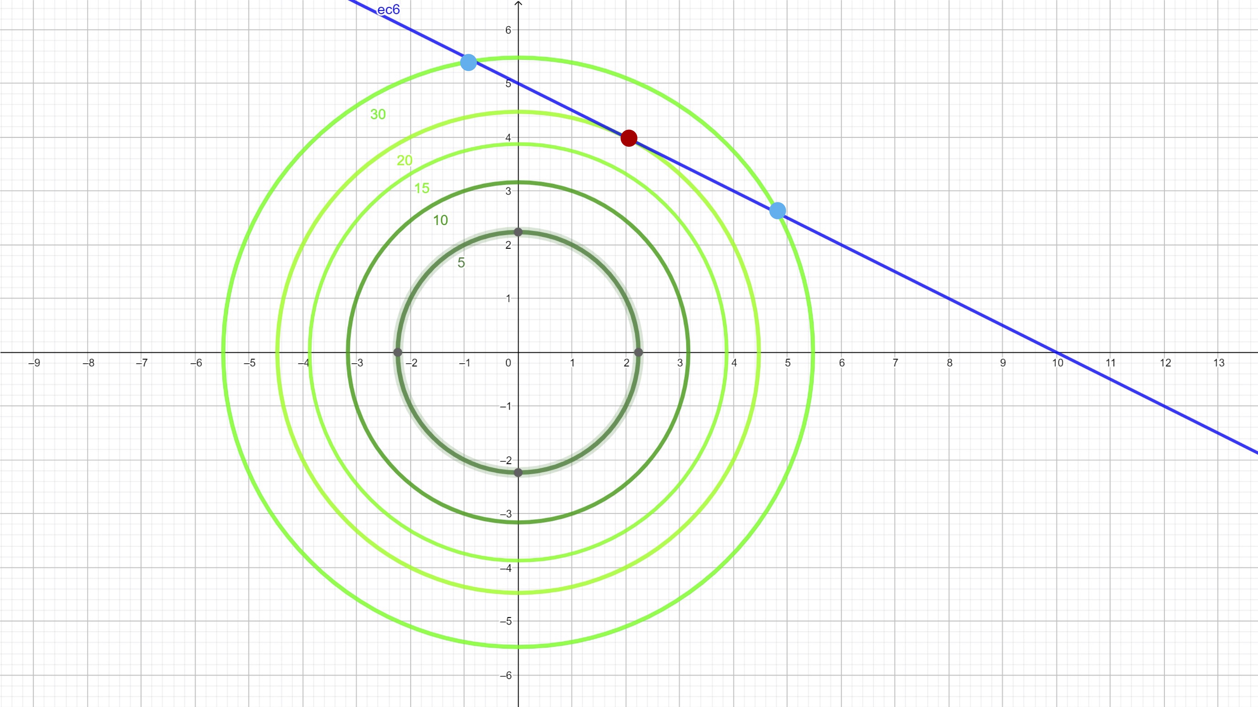
FIG 2 We also include three points of interest

As you can see, we have marked three points: the blue ones are feasible (since they satisfy the constraint) but give a value of the function target of 30. However, the red dot is feasible and gives a value of the target function of 20. Is there any feasible point (i.e. that is contained in the line) that gives a lower value of the function objective? No! Therefore, we have found the minimum (global) of problem. It’s at point \(x^{*}=2,y^{*}=4\).

Let’s continue analyzing the figure. Now, let’s calculate the gradient of the target function

\[ \nabla f(x,y)=\left[2x,2y\right] \]

and let’s draw it at the point that gives us the minimum of the problem (\(x^{*},y^{*})=(2,4)).\) The gradient turns out to be \[ \nabla f(2,4)=\left[4,8\right] \]

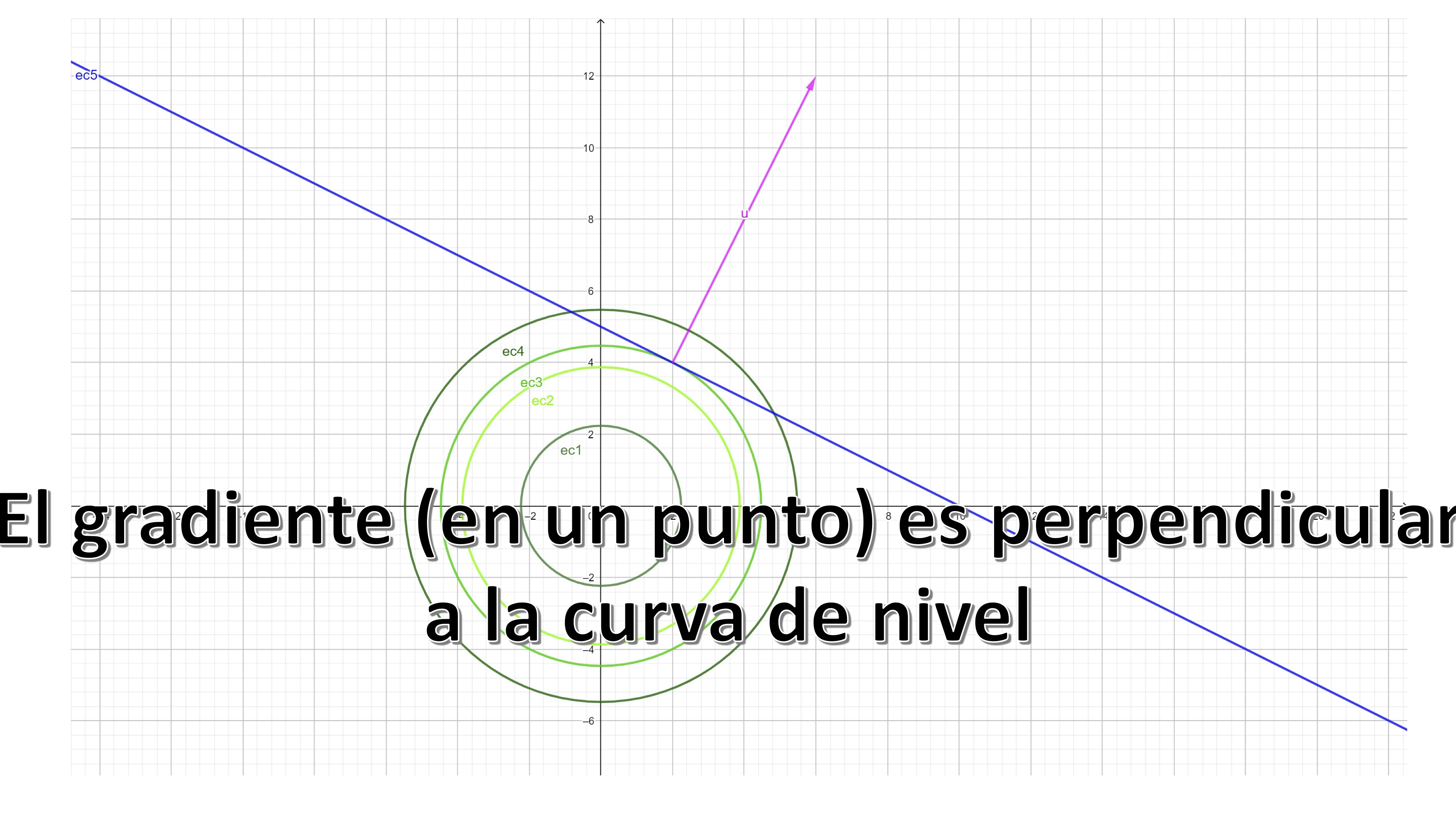
FIG 3 recalls that the gradient, at a point, is perpendicular to the contour at that point

Now, on the other hand, let’s get the gradient vector of the constraint. \(g(x,y)=x+2y\): \[ \nabla g(x,y)=\left[1,2\right] \] we draw it, likewise, and we obtain:

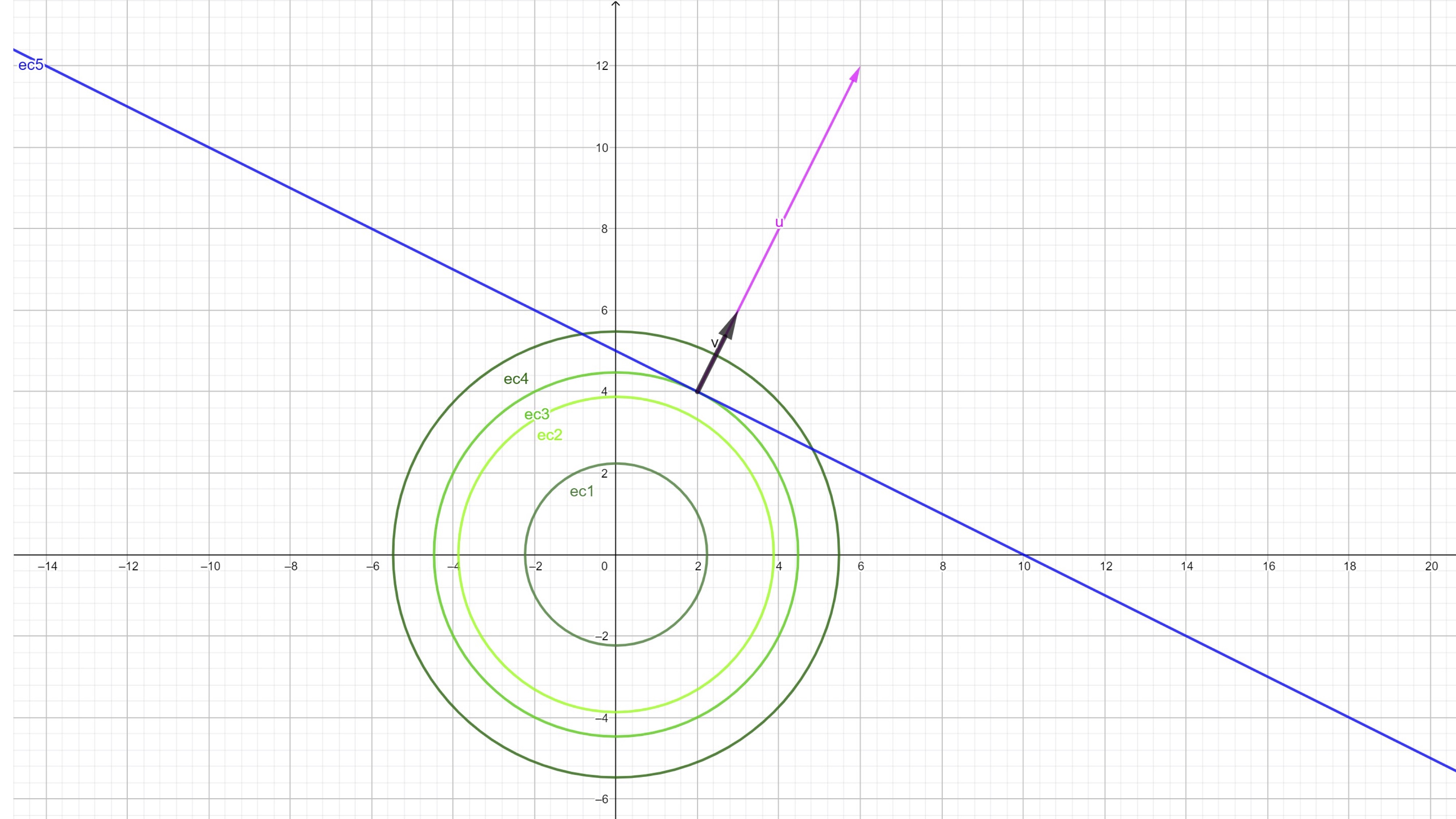
FIG 4 Both vectors are “proportional”

As you can see, they are proportional. Let’s think: could this same thing happen between others? pair of vectors that satisfy the constraint? You can try to see it graphically: impossible! Then, at the point where you get the global minimum both vectors are proportional, that is, it exists a \(\lambda\) such that:

\[ \nabla f(x^{*},y^{*})=\lambda\nabla g(x^{*},y^{*}) \]

in such a way, moreover, that the restriction is satisfied. The same thing Discovered Lagrange and devised a simple way to work through a function which encompasses both the objective function and the constraint: the “Lagrangian.” In an optrimization problem with equality restrictions:

\[ Opt_{x,y}f(x,y) \]

subject to: \[ g(x,y)=C \]

We define the Lagrangian, \(L(x,y,\lambda)\) as

\[ L(x,y,\lambda)=f(x,y)-\lambda\left[g(x,y)-C\right] \] and the first-order conditions are \[ \frac{\partial L}{\partial x}=0 \]

\[ \frac{\partial L}{\partial y}=0 \]

\[ g(x,y)=C \]

That is, to find critical points / candidates for optimal we must solve this system of equations.

• In this video you can delve deeper into the concepts developed by Lagrange

Example with the problem

We define the Lagrangian: \[ L(x,y,\lambda)=x^{2}+y^{2}-\lambda\left[x+2y-10\right] \]

we operate in the first order conditions \[ \begin{cases} \frac{\partial L}{\partial x}=0\Rightarrow2x-\lambda=0 & (1)\\ \frac{\partial L}{\partial y}=0\Rightarrow2y-2\lambda=0 & (2)\\ x+2y=10 & (3) \end{cases} \]

let’s solve this system of equations. For example, from (1) and (2), we have to: \[ 2x=\lambda \] \[ y=\lambda \] then \[ 2x=y \]

substituting in (3), we have to \[ x+4x=10\Rightarrow x^{*}=2 \] and, therefore, \[ y^{*}=4, \] and finally, \[ \lambda=4 \]

How do we know if it’s global? To do this, we will need to think about the constraints of the problem:

In this course, we will address two types of restrictions \(g(x,y)=C\): straight the curves:

Straights

if they are straight, as is the case we have just presented, Weierstrass’s Theorem is not fulfilled, since a line is not a bounded set.

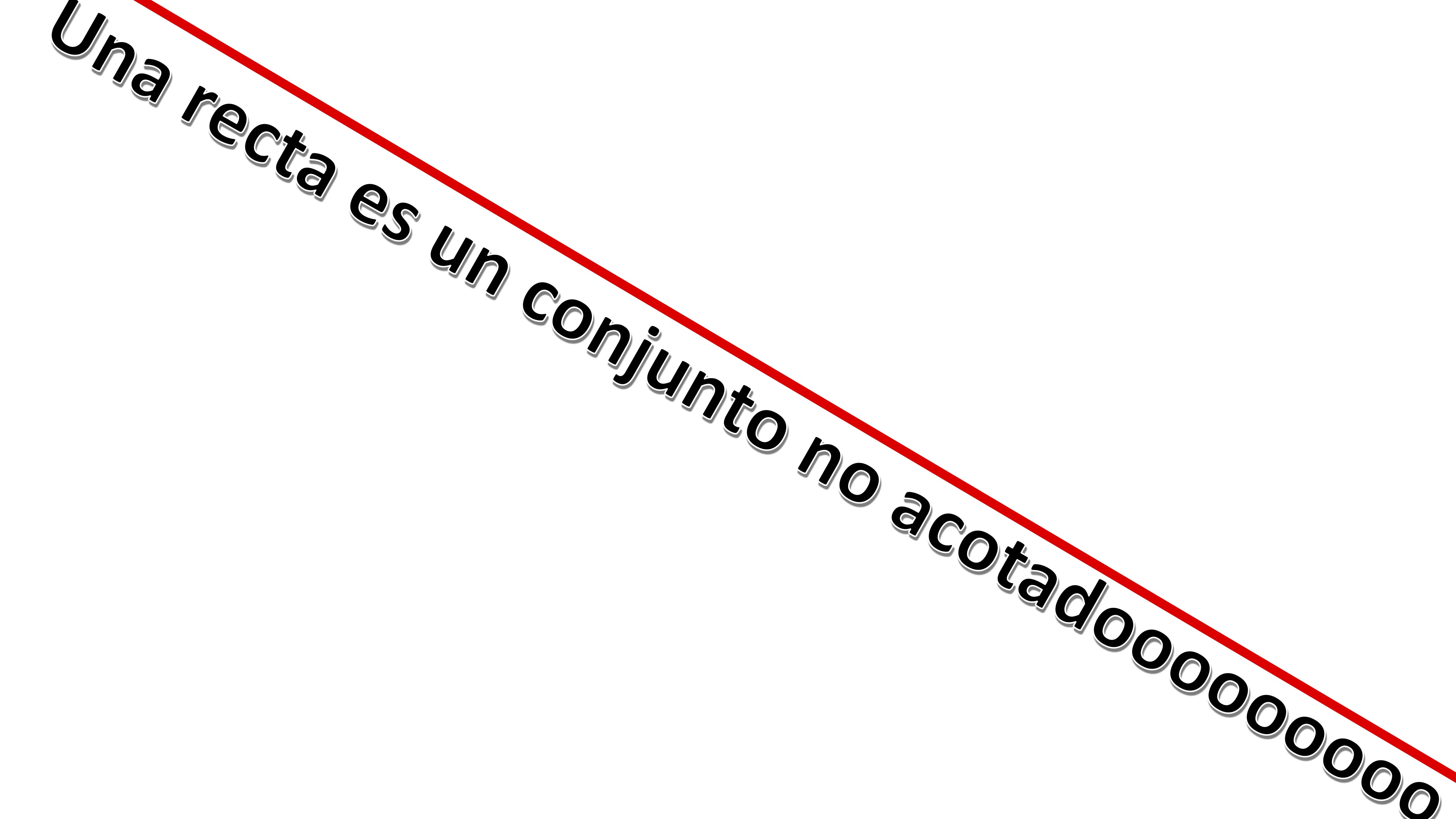
FIG 5 the lines are not “bounded”

However, being a convex set, we can use the Global Local Theorem (see in the previous class)

In this case, we analyze the Hessian of the objective function: \[ Hf(x,y)=\left[\begin{array}{cc} 2 & 0\\ 0 & 2 \end{array}\right] \] which, as you can see, is Positive Definite for all \((x,y)\) so this problem is of global minimum.

Curves

If the constraint (don’t confuse with contour lines) \(g(x,y)\) are circumferences or ellipses,

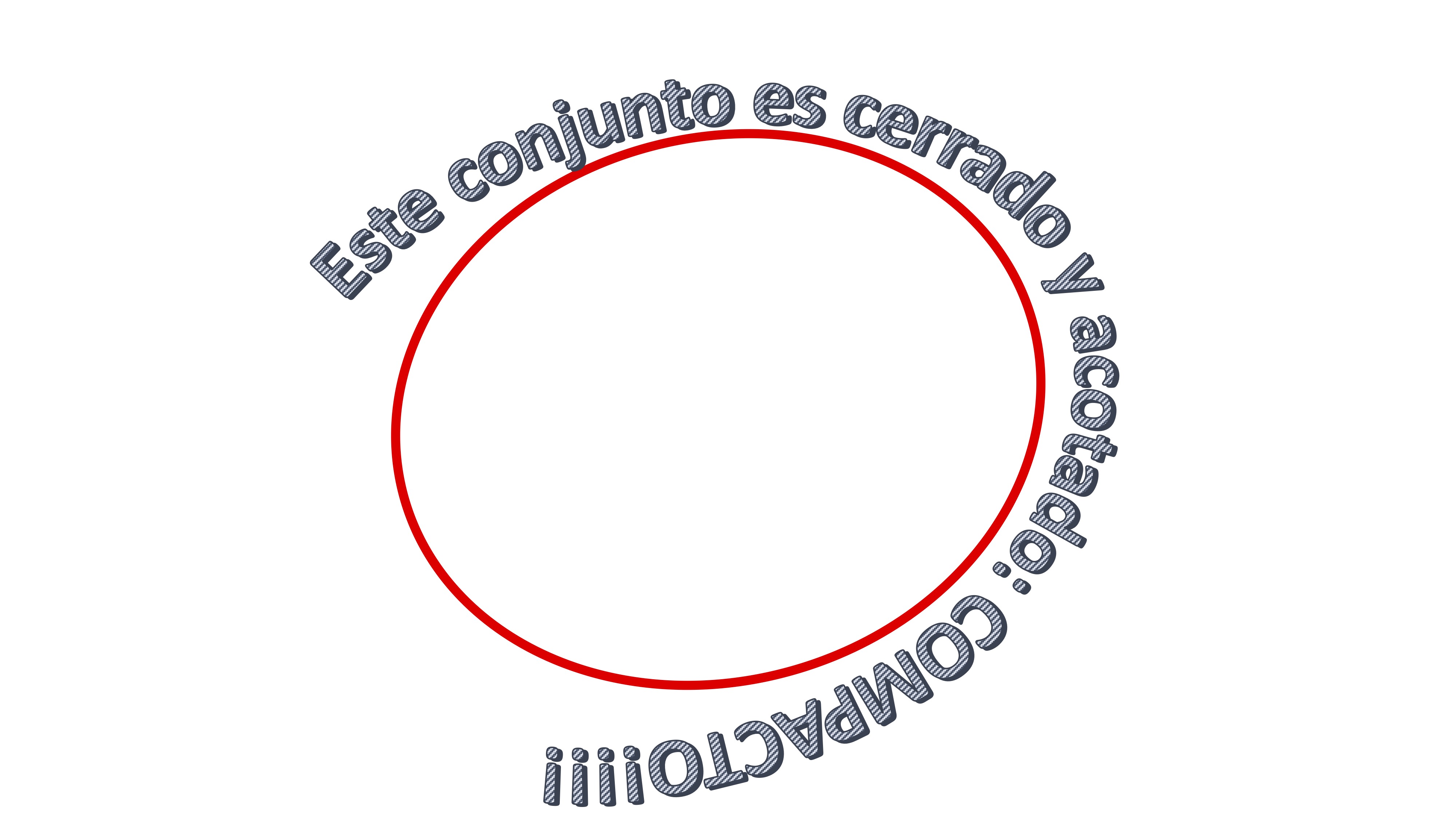
FIG 6 circumferences and ellipses make up a compact set

then the set is closed and bounded (compact) y, (as will be the case, the objective function \(f(x,y)\) is continuous) the Weierstrass theorem is satisfied. In that case, evaluate the function \(f(x,y)\) at critical points and classify them by following such values

Remember

Again you have to think in terms of

• Weierstrass
• Local-Global Theorem

Make an outline about all this you have learned, it will be easier for you to work.

• In this video we develop these ideas

Example: determines the points that verify the necessary conditions of the optimality of the problem:

\[ \min2x+3y \]

subject to \[ x^{2}+1.5y^{2}=6 \] \[ L(x,y,\lambda)=2x+3y-\lambda\left[x^{2}+1.5y^{2}-6\right] \]

CpOs are:

\[ \frac{\partial L}{\partial x}=0\Rightarrow2-2\lambda x=0 \] \[ \frac{\partial L}{\partial y}=0\Rightarrow3-3\lambda y=0 \] \[ x^{2}+1.5y^{2}=6 \]

The following system must be resolved: \[ \begin{cases} 2-2\lambda x=0 & (1)\\ 3-3\lambda y=0 & (2)\\ x^{2}+1.5y^{2}=6 & (3) \end{cases} \]

From equation (1) we have \(\lambda=\frac{1}{x}\) in the same way that of (2) we have that \(\lambda=\frac{1}{y}\). So, equalizing both equations \(\frac{1}{x}=\frac{1}{y}\Rightarrow y=x.\) Substituting in (3), we have to \(x^{2}+1.5x^{2}=6\Rightarrow2.5x^{2}=6\Rightarrow x^{2}=2.4.\) Then \(x=\pm1.55\) and, of course, \(y=\pm1.55\). We have two points Critical: \[ A(x^{*},y^{*},\lambda^{*})=\left(1.55,1.55,-0.645\right) \]

\[ B(x^{*},y^{*},\lambda^{*})=\left(-1.55,-1.55,+0.645\right) \]

It is very easy to see that \(A\) is the overall maximum and that \(B\) is the global minimum, evaluating these points in the target function.

Sufficient conditions of local optimum

Working with equality restrictions

• It is necessary to define the matrix “Hessiana Orlada”
• It will allow you to classify critical points as local maximum/minimum

To classify the critical points (in case of having several and Weierstrass is not met), we can use the criterion of the Hessian Orlado. We define the Ornate Hessian as

\[ \overline{H}L(x,y,\lambda=\left(\begin{array}{ccc} 0 & \frac{\partial g}{\partial x} & \frac{\partial g}{\partial y}\\ \frac{\partial g}{\partial x} & \frac{\partial^2 f}{\partial x^2} & \frac{\partial^2 f}{\partial x\partial y}\\ \frac{\partial g}{\partial y} & \frac{\partial^2 f}{\partial y \partial x} & \frac{\partial^2 f}{\partial y^2}\\ \end{array}\right) \]

If the determinant, at the candidate point, is greater than zero, then it is a local maximum and if it is less than zero, a local minimum.

In the videos and in the solved exercises you have examples of the use of the Ornate Hessian.