BLOCK 1: Modeling and visualization

• This block aims to pick up the baton to many of the mathematical ideas with which you have already worked in high school and primary. However, let’s give them a new approach: why don’t we try to make a function useful for us to make predictions (in the same way as it is done in the scientific world)? Why don’t we learn new ways of visualizing information in which several variables are involved?
• We will combine learning with inverted class sessions (that is, the student must work in the class prior to it, so that there can be discussion about the complicated points of the session and the proposed exercises) and master class (the teacher will develop the key ideas in a more traditional class)
• This text (which should not replace a good calculus book) is a reference as class notes that, in addition, contains links to youtube videos prepared by the author to motivate and reinforce ideas

References of interest

• Stewart, J. (2009). Calculus: Concepts and contexts. Cengage Learning.
• STEWART, James; CLEGG, Daniel K.; WATSON, Saleem. Calculus: early transcendentals. Cengage Learning, 2020.
• SYDSAETER, Knut; HAMMOND, Peter. Mathematics for economic analysis. Pearson Education, 1996.
• SIMON, Carl P., et al. Mathematics for economists. New York: Norton, 1994.
• SMITH, Robert T.; MINTON, Roland B.; RAFHI, Ziad AT. Calculus of several variables: early transcendents. McGraw-Hill Interamericana, 2019.

Class 1 (inverted): the concept of function in \(1\) and \(n\) variables

Inverted class!

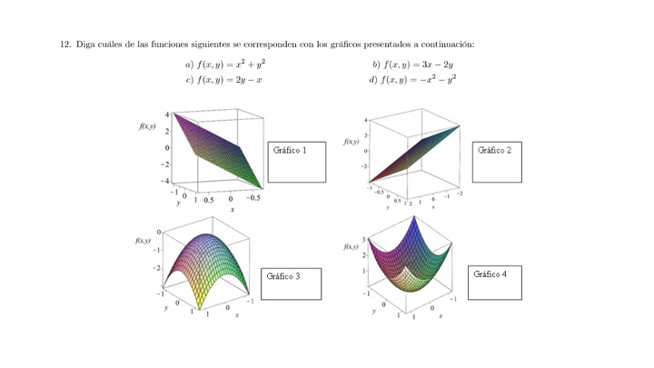
This is an inverted class session. You should watch the video you have below and try to make the exercises. In the classroom, what has been learned will be discussed and the concepts that are not clear will be expanded. This is because much of what you are going to learn new is an extension of what you should already know.

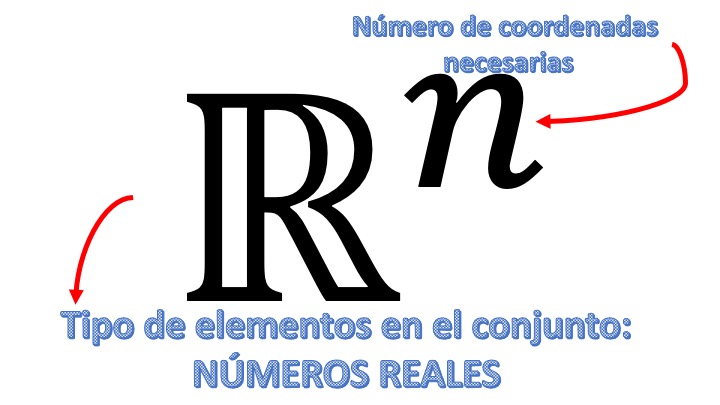
A function is a rule (usually called \(f,g,h,....\)) that assigns to the values of a set called domain a single the value of an assembly named image. In this course we will work, in general with functions \(\mathscr{\mathbb{R}}^{n}\rightarrow\mathbb{R}\), indicating that the domain is a \(n-\) dimensional set of numbers real (very often \(n=1.2\)) and \(\mathbb{R}\) is the famous real line.

• Make sure you understand what \(\mathbb{R}^{2}\) and \(\mathbb{R}^{3}\) mean.
• Are you convinced by the video?

In this course we will work, in general, with the real numbers \(n\) dimensional, which is already an advance compared to what you have learned in past courses.

[]

Ejemplo of a function of a variable: Let be the function \[ f(x)=\frac{1}{x-1} \] As you can see, the domain is all real values except 1, since whereas the function, when the denominator is worth 0, is not defined; and we write it like this \[ D=\left\{ x\in\mathbb{R}|x\neq1\right\} \] The path (or range, or image) are the possible values that can take the \(y.\) In this case, it will be all \(\mathbb{R}\) except the value 0.

You can use Geogebra to make the graphs for many of the functions to be presented in this course. For example, here we represent the above function:

FIG1. The real function of real variable of Annotation 1 would you know how to do it by hand?.

If we have \(n\) variables, which is the new thing about this course, the idea will be similar: we need a rule that assigns a single output to a set of \(n\) input variables.

Función of n variables: A function of variables is defined as \[ y=f(x_{1},x_{2},...,x_{n}) \]

\(y\)	\(x_{1},...,x_{n}\)
endogenous	exogenous
explained	explanatory
	dependent independent

And we need \(n\) variables because the models you will study in Social sciences are usually based on a broad set of factors that explain a fact. Then:

We say that \(f\,:\,D\subset\mathbb{R}^{n}\rightarrow\mathbb{R}\) if the rule or function \(f\) assigns to each value in the domain \(D\) (which is a subset of the real numbers \(n\) dimensional) a value real. In this text we will use, generally, functions of two variables, I mean:

\[ y=f\left(x_{1},x_{2}\right), \]

donde \(f\,:\,D\subset\mathbb{R}^{2}\rightarrow\mathbb{R}.\)

But of course, we could have a variable \(n\) function.

\[ y=f\left(x_{1},x_{2},...,x_{n}\right), \]

donde \(f\,:\,D\subset\mathbb{R}^{n}\rightarrow\mathbb{R}.\)

Ejemplo: think about the functions that appear in the vídeo: \[ ResultsPISA=f(expenditure) \] is a function \(\mathbb{R\rightarrow R}\), on the other hand, \[ BMI=\frac{weight}{height^{2}} \] is a function \(\mathbb{R}^{2}\rightarrow\mathbb{R}\), while the last function

\[ M=C_{0}\frac{\left(1+\frac{i}{m}\right)^{n\times m}\left(\frac{i}{m}\right)}{\left(1+\frac{i}{m}\right)^{n\times m}-1} \]

is \(\mathbb{R}^{4}\rightarrow\mathbb{R}\). Make sure you understand what this means, according to what is said in the video.

[]

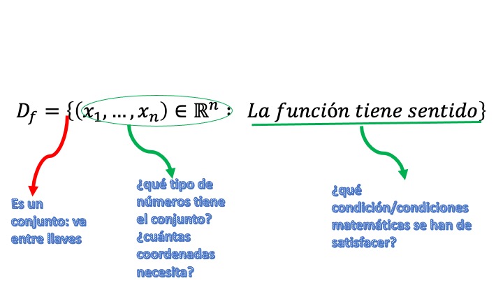
The domain of a function is the set of values of the variable(s) independents for which the function is defined and makes sense.

-If the function is \(f\::\:\mathscr{\mathbb{R}}\rightarrow\mathbb{R},\) (for example, \(y=f(x))\) the domain can be written as \(D=\left\{ x\in\mathbb{R}\::\:f\;\mathrm{est\acute{a}\:d efinida}\right\}\).

What you’re saying is that _el domain consists of values. of the variable \(x\), such that they belong to the set of numbers real, as long as the function has sentido matemático. Where put f is definida, you must put what conditions it must comply for it to be. For example, \(y=ln(x+1)\), \(D=\left\{ x\in\mathbb{R}\::\:x>-1\right\}\).

-If the function is \(f\::\:\mathscr{\mathbb{R}}^{2}\rightarrow\mathbb{R}\), (for example, \(y=f(x_{1},x_{2}))\), the domain is written as \(D=\left\{ (x_{1},x_{2})\in{\mathbb{R}^{2}}\::\:f\;\mathrm{is\:d efinida}\right\}\). For example, \(y=ln(x_{1}+x_{2})\), \(D=\left\{ (x_{1},x_{2})\in\mathbb{R}^{2}\::\:x_{1}>-x_{2}\right\}\).

Notice how we indicate \(\mathbb{R}^{2}\) as the set where we are going to find the values for the independent variables.

• If the function you’re working with makes economic sense, physical, biological,… it is convenient that you think about possible additional restrictions in the domain, indicating that you will use such restriction.

You can call it natural Dominio or Económico (for example, if the function demand for a good depends on two prices, \(y=-2x_{1}+3x_{2}\), then \(D_{N}=\left\{ (x_{1},x_{2})\in\mathbb{R}^{2}\::\:x_{1},x_{2}>0\right\}\), mientras que \(D=\left\{ (x_{1},x_{2})\in\mathbb{R}^{2}\right\}\), since there are no negative prices (natural domain) but the function would make mathematical sense for any real value of exogenous variables.

In the previous video appears another function of two variables very famous, that you know, and that -maybe- you do not you had stopped to think that it was: the body mass index.

FIG 2. This is the BMI you find in the pharmacy. In the exercises we will work on it.

Body mass index (BMI) is a function that has its dominance in two dimensions (the pair \((p,a)\)) and whose image is a single real value (the index value for each individual). That is, \(f\::D\subset\mathbb{R}^{2}\rightarrow\mathbb{R}:\)

\[\begin{equation} IMC=\frac{p}{a^{2}} \tag{1.1} \end{equation}\]

In this case, the function can be written as follows:

\[ IMC=f(p,a) \]

If you notice, the variable output or endogenous is the BMI, while \(p.a\) are the inputs or exogenous of the function. Belong to values in \(\mathbb{R}^{2}\). But will any stop in \(\mathbb{R}^{2}\) be valid? For example, is it worth saying that the weight of an individual is -15 kg and his height -1.75 meters?

What will be the domain? In principle, if we analyze the function in a cold way without knowing what is \(p\) or \(a\), we have to think about what function values would make it incorrect Defined. In this case, if \(a=0\), the BMI will not be defined, since we cannot divide by zero. So the domain of the function Be:

\[ D=\left\{ \left(p,a\right)\in\mathbb{R}^{2}|a\neq0\right\} \]

(which reads: the domain of the function is the set of all real values in two dimensions of \(p\) and \(a\) such that \(a\neq0\))

However, this domain doesn’t seem to make sense. Can be the weight of an individual -8 kilograms on planet Earth such and how are things? NO! Therefore, we define the natural domain of a function that will be the one that makes economic sense, in a broad way (by economic we also mean social, psychological, biological, etc …). In our case, since weight and height are always values positive, the natural domain:

\[ D_{N}=\left\{ \left(p,a\right)\in\mathbb{R}^{2}|p>0,a>0\right\} \]

Therefore, the domain, in the end, is the subset of the real numbers \(n\)-dimensional (in this case, \(n\)=2) for which the function makes sense. The range (route or image) will be sought in the set: \(\mathbb{R}\)). The image is the result of applying the expression of the function to the set of \(n\) values that belong to the domain.

FIG3 This is the schematic idea of BMI. The domain is in two dimensions, while the image is in one dimension.

1.3.1 What do we need the functions for?

As noted in the video, in general the functions are a tool very natural to be able to express a human, economic behavior, social, health, etc … They allow to provide logic to a model with the goal of being able to obtain predictions. Think that one of the greats The purpose of science is to be able to tell what is going to happen. and, in addition, to have tools to optimize results. You can make this short reading that, as you will see, has a lot of current

https://theconversation.com/covid-19-pandemia-de-modelos-matematicos-136212

Exercise 1

Think, or search the internet, in contexts where you think function-based mathematical models are used. Propose any in class.

Exercise 2

The following graph shows several curves in the drawing. Identifies which correspond to functions of the form \(y=f(x)\), which correspond to functions of the form \(x=f(y)\) and if, by some modification (to the domain), some function can be extracted from where, in principle, there is none.

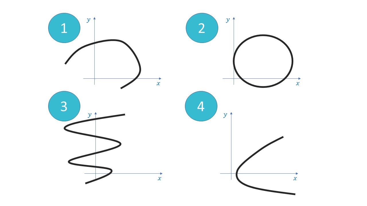
Chart for Exercise 2

Exercise 3

The following diagrams propose different possible functions. the direction of the arrow indicates which is the domain and which is the set image (\(dominio\rightarrow image)\). Discuss whether or not they are functions and under what conditions (for example, a restriction on the domain) can be:

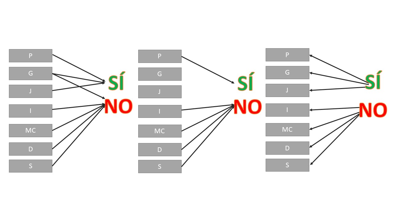
Chart for Exercise 3

Exercise 4

Find the domain and image of the following functions:

1. $h(t)=t^{3}+t{2}+$1

2. \(f(x)=\sqrt{10-2x}\)

solución \(D_{f}=\left\{x\in\mathbb{R}\::\:x\leq5\right\}\), \(Im_{f}=[0,\infty)\)

3. \(y(k)=\frac{2k-1}{k^{2}-k}\)

4. \(j(x)=\sqrt{9-x^{2}}\)

5. \(g(p)=\left(\frac{p-1}{\left(p-2\right)\left(p-3\right)}\right)^{1/2}\)

Exercise 5

Let \(W(q)\) be the function defined by

\[ W(q)=\frac{3q+6}{q-2} \]

• Calculate your domain
• Shows that 5 belongs to the image set of the function Is also the 3 in that set?

Exercise 6

Find the domain of the following functions defined in \(\mathbb{R}^{2}\rightarrow\mathbb{R}\)

1. \(f(x,y)=x-3y\)

2. \(g(x,y)=\ln(x-3y)\)

solution \(D_{g}=\left\{ (x,y)\in\mathbb{R}^{2}\::\:x-3y>0\right\}\)

3. \(h(x,y)=x+4y^{2}\)

4. \(i(x,y)=\frac{x}{y-2}\)

5. \(j(x,y)=4(x-1)^{2}+9(y-2)^{2}\)

6. \(k(x,y)=(x-1)^{1/2}(y-2)\)

7. \(l(x,y)=\ln y+x\)

8. \(m(x,y)=\ln(y+e^{-x})\)

Exercise 7

The function \(x(p,q)=\frac{20-p+q}{p}\) represents the demand \(x\) of a good, given its price \(p\) and the price of another good, \(q\). Finds your natural (or economic) domain and draw the \((p,q)\) points of the natural (or economic) domain for which the demand is greater than or equal to 3 units.

-Indication for the second part: you must solve \(\frac{20-p+q}{p}\geq3\) and draw the inequality you find. You can check it with Geogebra

Solved Exercise

Imagine a function \(f\), whose domain is made up of weight and the height of an individual and the image is the BMI of the individual and, in addition, it takes the following values:

• 0, if the individual is at their weight
• 1, if the individual is overweight
• -1, if the individual has a lower than normal BMI.

Explain what the domain and image of the function would look like. Reason if it is a function defined as \(f\::\mathbb{R}^{2}\rightarrow\mathbb{R}\). If not, it specifies the function appropriately. Search in addition, a sensible way to give the result for an individual whose Weight is 68 kilograms and its height is 1.80 meters.

solution:

the function is not of type \(f\::\mathbb{R}^{2}\rightarrow\mathbb{R}\) but of this other \(f\::\mathbb{R}_{++}^{2}\rightarrow\mathbb{R}^{2}\), Caution!! this does not mean that you have two images in the same set. You have an image in the BMI set and another in the \(\left\{ 0,1,-1\right\}\) set that evaluates your result. The function is such that \[ D=\left\{ (p,a)\in\mathbb{R}_{++}^{2}\right\} \]

\[ Im=\left\{ (IMC,y)\in\mathbb{R}^{2}\::\:IMC>0,y=\left\{ -1,0,1\right\} \right\} \] So \(f(68,1.80)=(20.98,0)\).

Exercise 8

Expresses the natural domain of the following function being spoken of in video 1, found in Ponferrada (León). To do this, come back to the video, look at the details of each variable and think about which set it is well defined.

\[ M=C_{0}\frac{\left(1+\frac{i}{m}\right)^{n\times m}\left(\frac{i}{m}\right)}{\left(1+\frac{i}{m}\right)^{n\times m}-1} \]

Remember the sets of numbers we know:

Natural: to count. \(\mathbb{N}=\{0,1,2,3,....\}\)

Integers: an extension of the natural \(\mathbb{Z}=\left\{....,-3,-2,-1,0,1,2,3,....\right\}\)

Racionales: \(\mathbb{Q}=\left\{\frac{p}{q},p\in\mathbb{Z},q\in\mathbb{Z}\setminus\left\{ 0\right\} \right\}\)

Irracionales \(\mathbb{I}=\left\{e,\pi,\sqrt{2},...\right\}\)

Reales \(\mathbb{R}=\mathbb{N}\cup\mathbb{Z}\cup\mathbb{Q}\cup\mathbb{I}\)

Class 2 (magistral): review of graphs real variable functions (I)

The simplest function you’ve worked with in all your previous education is the straight one:

\[ y=ax+b \]

where the \(y\) is the dependent variable and the \(x\) is the variable independent.

How is $$b interpreted?

It is the ordered one at the origin. It is the value of the \(y\) when \(x=0\).

How is $$a interpreted?

It’s the slope. How much does \(y\) change in the face of \(x\) increases in a unit.

• If \(a>0.\) the increase of \(y\) against increases of \(x\) is positive (\(x,y\) are proportional)
• If \(a<0.\)el increase of $ $y against increases of $ \(x is negative (\)x,y$ are inversely proportional)

What is it used for in Economics?

When we want to make simple models to understand the, complex and difficult to know in detail, reality.

The equation of a line can be obtained depending on the information provided to us

Name	information I am given by	Equation
point-slope	\(a,(x_{0},y_{0})\)	\(y-y_{0}=a(x-x_{0})\)
Two points	\((x_{0},x_{1}),\left(y_{0},y_{1}\right)\)	\(y-y_{0}=\frac{y_{1}-y_{0}}{x_{1}-x_{0}}(x-x_{0})\)
Intersection with	axes \(x=a,y=b\)	\(\frac{x}{a}+\frac{y}{b}=1\)

We will say that two lines \(y=c+m_{1}x\), \(y=d+m_{2}x\) are parallel if the slopes are equal (\(m_{1}=m_{2})\). They are perpendicular if the product of your earrings is -1 \((m_{1}m_{2}=-1)\). Draw, in geogebra two parallel and perpendicular lines and make sure that it is fulfilled.

Exercise 1

Find the slope and the ordered one at the origin of the following lines. Dibújalas.

1. \(20x-24y-30=0\)

2. \(2x-3=0\)

3. $4y+5=$0

-Write an equation for a line that passes through the point \((-3,2)\) and that is parallel to \(3x-5y+8=0\). Draw them.

-Write an equation for a line that passes through the point \((2,-4)\) and is perpendicular to \(x-4y+8=0\). Draw them.

-A point \(A\) is collinear to a line \(r\), if the point is in the line (\(A\subset r).\) Study whether the following points are collinear: \(A(-5.3),B(-1.8),C(3.0).\) Find a way to find two points collinear to any line.

Class 3 (magistral): review of graphs real variable functions (II)

Polynomial functions

Parable. \(y=ax^2+bx+c\). We have two cases

\(a<0\) shaped: \({\color{red}\cap}\)

\(a>0\) shaped: \({\color{teal}\cup}\)

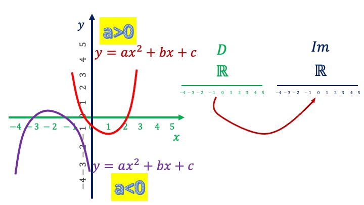
The Parables

Remember

• vertices: \(x=\frac{-b}{2a}\) \(y=f(\frac{-b}{2a})\).
• cut with the axis of the \(x\) : \(\frac{-b\pm\sqrt{b^{2}-4ac}}{2a}\)
• cut with the axis of the \(y\), we make \(x=0\) and obtain the corresponding value.

cubic. \(y=a+bx+cx^{2}+dx^{3}\). We have two cases

\(d<0\) with form: \({\cup\cap}\)

\(d>0\) with form: \({\cap\cup}\)

[The Cubics] (Diapositiva4_2_ceu.jpg)

Later, when we see applications of derivatives, we will see how to draw them more accurately. It is true that the drawing of polynomial graphs is complicated with the degree of the polynomial and it is necessary to know more Calculus tools to do it properly.

Potentials . Functions of type \(f(x)=x^{n}\). With different types of values for \(n\). Look at the footers of each of the images to identify them

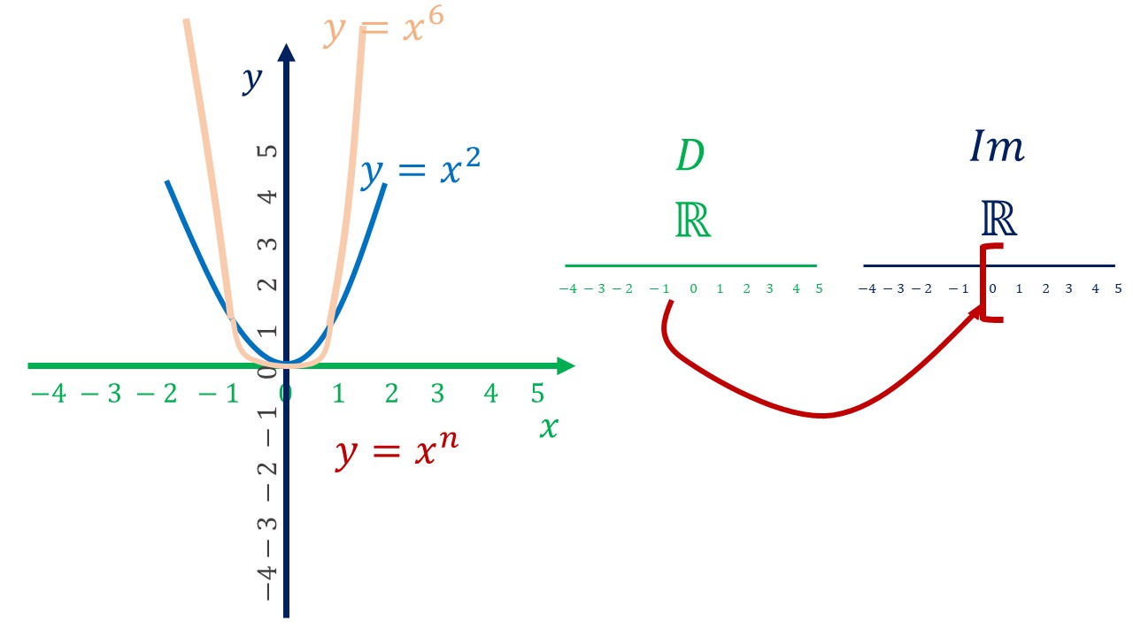
\(n\) even and positive , \(n=\left\{ 2,4,6,....\right\}\)

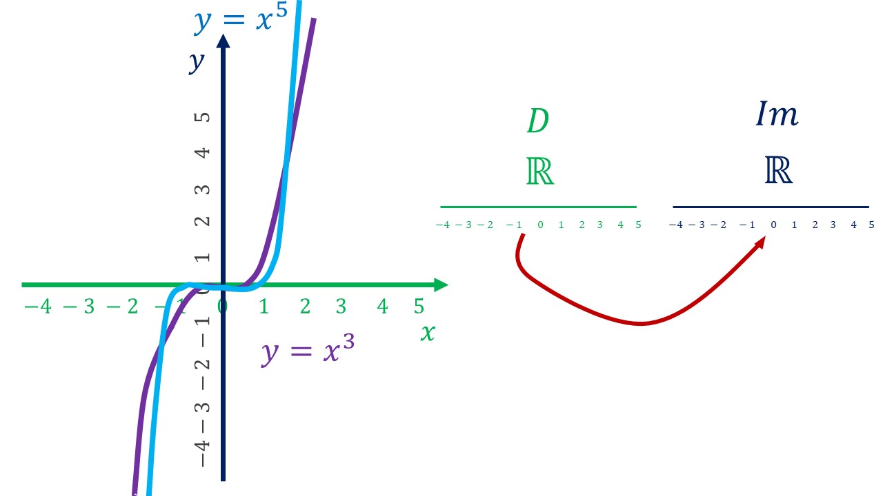
\(n\) odd and positive , \(n=\left\{ 3,5,7,....\right\}\)

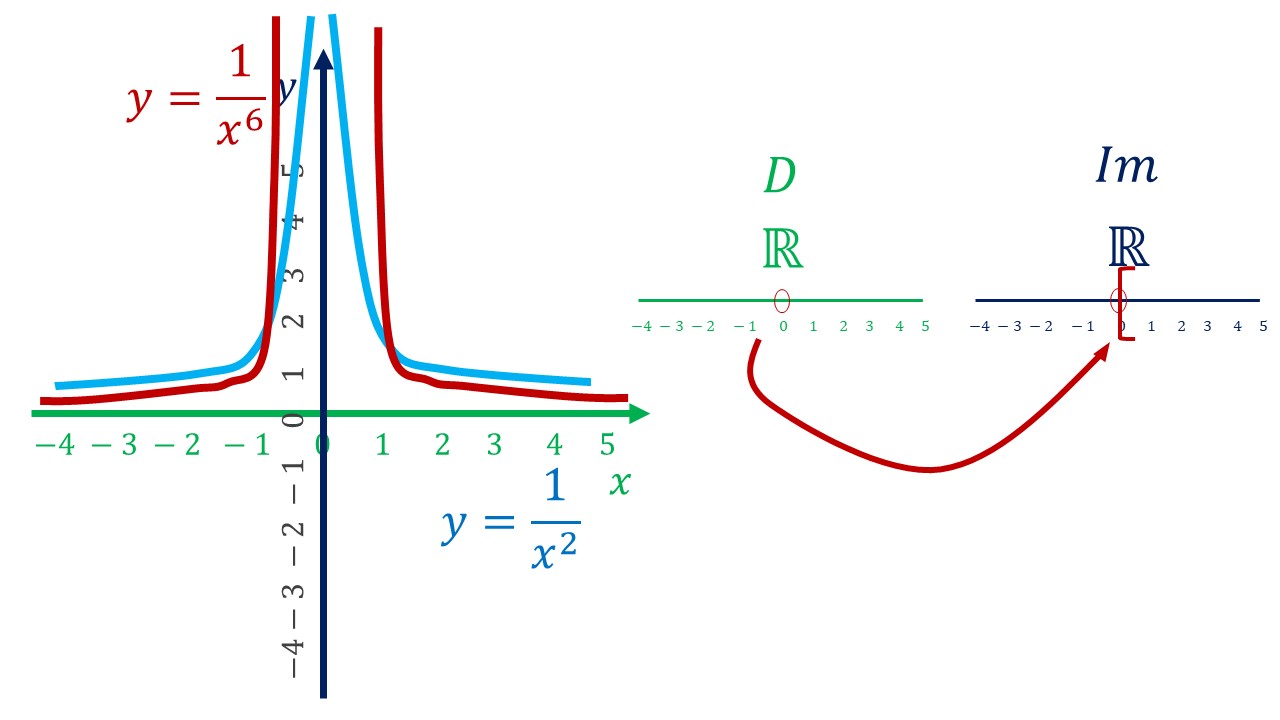
\(n\) even and negative , \(n=\{-2,-4,...\}\)

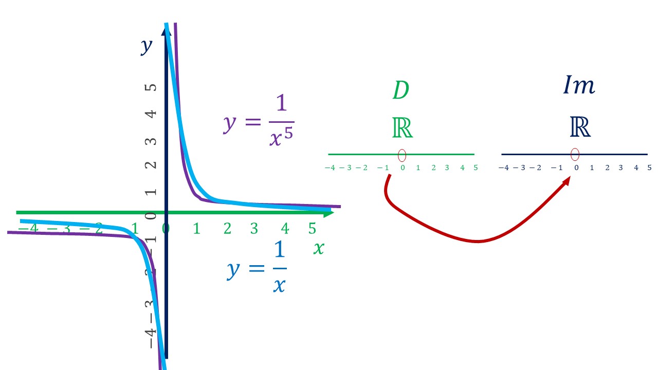
\(n\) odd and negative \(n=\{-1,-3.-5...\}\)

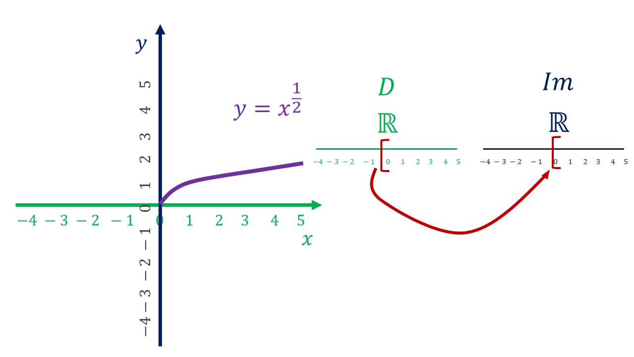
\(n\) positive and rational

In this video you can review ideas of these polynomial functions that we have presented to you

Exercise 3

Let be the function \(f(x)=ax^2+bx+c\). Knowing that the points \((1,-3)\), \((0,-6)\), \((3,15)\), are points of your graph: calculate the values of \(a,b,c\)

Exercise 4

Draw the graphs of \(f(x)=x^2\), \(g(x)=(x-2)^2\), \(h(x)=x^2+3\) How are these graphs related?

Exercise 5

A very convenient way to write a parable is like this: \(y=(x-2)(x-8)\) Why? it already gives us the roots of the second-degree equation! Draw it.

Exercise 6

write in a simplified way and then draw the following potential functions

• \(f(a)=(((a^{1/2})^{2/3})^{3/4})^{4/5}\)

• \(g(x)=(((3x)^{-1})^{-2}(2x^{-2})^{-1})/x^{-3}\)

Logarithm and exponential

The logarithm - based on \(a\) - is a function such that

\[ log_{a}y=x\Longleftrightarrow a^{x}=y \]

This relation further indicates that the function inverse to the logarithm is the exponential function (and vice versa): \[ y=a^{x} \]

Where \(a>0\).

It is very common to use the logarithm in base \(e\), that is, the Neperian logarithm. In such a way that

\[ \ln y=x\Longleftrightarrow e^{x}=y \]

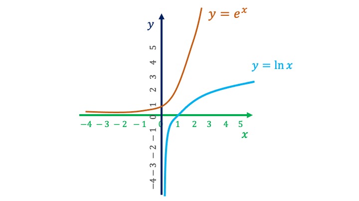
In this figure you can see the property that both functions are inverse

Exercise 7

Retrieves the properties of the logarithm and the exponential. Make a list of them and always have it at hand.

Exercise 8

A savings book with an initial capital of $600 euros, produces a \(3\)% annual interest

Write a function that represents the capital that will be obtained in the year \(t\) and answer

• a: How long will it take for you to receive $655.63 euros?
• b: What happens to capital if $t becomes “very large?”

Exercise 9

After defusing a bomb, Special Agent 00.0 returns home and learns that his best friend “Siggy” has been killed. Police say the body was found at 1 a.m. on Thursday, in a refrigerator at 10ºF. He was also told that the temperature of the corpse, when it was found, was 40ºF. It is known that the temperature of a body, after death, follows function

\[ T=T_{a}+(98.6-T_a)(0.97)^t \]

Where \(T_a\) is the temperature of the air surrounding the body and \(t\) are the hours. The agent knows that the murder was committed either by Ernest Stabros or by André Scélérat. If the former was in jail until Wednesday and the latter was seen in Las Vegas from noon Wednesday through Friday: who committed the crime?

hint: you need to get $$t for the data you have

Exercise 10

Demonstrates the following equalities

• a: \(ln(x)-x=ln(x/e^{x})\)
• b: \(ln (x) - ln(y) + ln(z) =ln(xz/y)\)
• c: \(3 +2ln(x)=ln(e^{3}x^2)\)

Simplify the following expressions

• a: \(e^{lnx}-ln{e^x}\)
• b: \(ln(x^4 e^{-x})\)
• c: \(e^{ln{x^2}-2ln{x}}\)

One of its uses is to simplify the units and scales of measurement. By Example, look at this information from El País on the Coronavirus data:

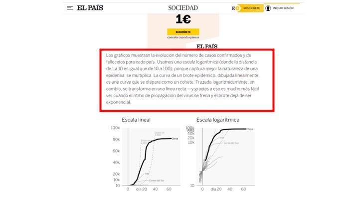
the logarithm is in the press!

What this press clipping means is that if the virus advances following an exponential function such as this \(f(x)=ae^{bx}\), with \(a,b\in \mathbb{R}\), if the logarithmic transformation is introduced to the data, it should become a line. See how:

\[ y=ae^{bx} \]

\[ \ln y=\ln a+\ln e^{bx} \]

\[ \ln y=\ln a+bx \]

\[ \ln y=a^{*}+bx, \]

In this video you have a good summary of the logarithm and exponential functions

Conical

The essential conics we will need this year are going to be circumferences and ellipses. Both are curves that are drawn in the plane (in \(\mathbb{R}^2\)) but that, as you can see, do not constitute a function (you would know why?) See? This is an example, of many, of a “formula” that is not a function.

circumference . Its canonical expression is \((x-x_{0})^2+(y-y_{0})^2=r^2\), so that \((x_{0},y_{0})\) is the central point of the circumference. The equation says that all points equidistan from it at the same distance, called \(r\) or radius. Therefore, drawing a circumference with this expression is very simple: you have both the center and the radius. It has no loss.

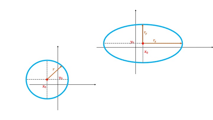
The circumference and ellipse

ellipse . Its canonical expression is \(\frac{(x-x_{0})^2}{r_x^2}+\frac{(y-y_{0})^2}{r_y^2}=1\), so that \((x_{0},y_{0})\) is the central point of the ellipse. As you already know, an ellipse is a “flattened” circumference. To draw it, you need to know its center again and, in the denominator of the expression \((x-x_{0})^2\) you will find the square of the semi-major axis (that is, \(r_x\)), while in the denominator of \((y-y_{0})^2\) you will find the square of the semi-minor axis (that is, \(r_y\)). With that information you can draw it as in the figure. It is important that you note that *the equation must be equal to 1. If not, you will need to divide on both sides by the same value.

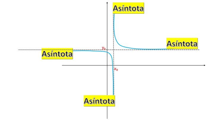
Equilateral hyperbola

equilateral hyperbola . Finally, another of the conics of interest. This is a function whose expression is \((x-x_0)(y-y_0)=K\), where \(K\) is a constant. It has, as well as asymptotes, the lines \(x=x_0\) and \(y=y_0\). And it is placed in the first and third quadrant if \(K>0\) and in the second and fourth if \(K<0\)

In this video you have a good summary of the conics. In addition, there are solved exercises that will help you practice.

• Caution!, all these graphs are not only relevant to this part of the course, but we will need them again to draw contour lines and, in addition, in Mathematics II.

Class 4 (inverted): modeling to answer questions

Inverted class!

This is an inverted class session. You should watch the video you have below and try to make the exercises. In the classroom, what has been learned will be discussed and the concepts that are not clear will be expanded. This is because much of what you are going to learn new is an extension of what you should already know.

Exercise 1

From the model presented in minute 1.30 of video 5:

\[ Hope\:d e\:life=a+b\times a\tilde{n}o\equiv y=a+bx \]

calculates the value for \(a\) and \(b\) using the points \((x_{0},y_{0}),(x_{1},y_{1})\equiv(1948,66.3)(2019,81.3)\). Discusses why \(a\) is different from the one obtained in the video, but \(b\) is the same. Do you get the same life expectancy prediction? by 2039? Justify why.

Exercise 2

Anthropologists use a linear model to relate length of the human femur with the height of the individual. This is important, since it allows, before the partial discovery of a skeleton, to predict the height of the individual. Use the following data to provide a model that allows us to make such a prediction (you can do it with Excel, for example, or a mano).

Femur Length	Height
50.1	178.5
44.5	168.3
48.3	173.6
42.7	165
45.2	164.8
39.5	155.4
44.7	163.7
38	155.8

Archaeologists working in Pompeii, when they found a petrified horse

• An individual has a femur with length 43 cmts What approximate height Have?
• An individual with femur length 58 ctms is found with a height of 180 ctms. What does this result suggest about the use of the model?

(Adapted from Stewart)

Exercise 3

Now you must give values to the parameters of the function that allows us to obtain life expectancy at birth according to the year (In this case, $a,b,c,d… $), using the data available in the Excel file, and the following function defined in chunks

\[ f(x)=\begin{cases} f_1(x) & x<1900\\ f_2(x) & x\geq1900 \end{cases} \]

a function where \(x\) is the year and \(f(x)\) is life expectancy. Analyzes:

• Whether or not it is continue the function you have found.
• If it is not continuous, reformulate \(f(x)\) and parameterize it to let it be.

• Discusses the appropriateness of using this model to predict hope of life in 1300, for example, and in the year 2100.

Exercise 4

A company that offers loans in 24 hours uses a granting of loans based on two variables of interest of the individual candidate to receive the loan: the months that he has been hired in the current company and his payroll. On base to the repayment of loans in the last year, they have made the next chart:

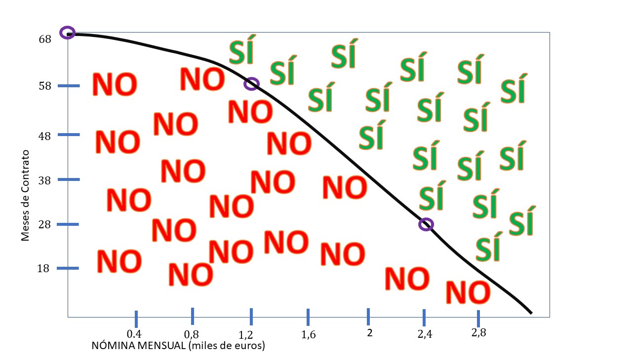
Marketing Company Sample

in such a way that it DOES indicate the characteristics (months of contract and salary) of the individual who repaid the loan and NOT, the opposite.

• Look for the function that relates months of contract and salary. Use that function (curvilinear) to determine the months of contract an individual needs so that, charging 1278 euros per month, the loan is granted.

• Marketing managers consider that the decision rule it is too strict and penalizes too many customers. Find another somewhat more permissive rule (a straight) and determines the contract months you would need an individual who charges 1278 euros per month to be granted the loan. If that rule had been used in the past, what percentage of individuals would have been defaulted despite granting them the loan?

A competing company has this other sample.

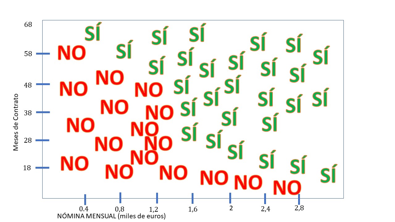
Marketing Company Sample

Could you define a function in such a way that it discriminates perfectly? yeses and noes?

Class 5 (masterful): contour lines

Once we have remembered how to represent real functions of real variable (remember that they are functions that have an explanatory variable and that are represented in a space of 2 dimensions), now we will see how to represent a function with two variables. Let’s go back to BMI, which you remember, writes

\[\begin{equation} IMC=\frac{p}{a^{2}} \tag{1.1} \end{equation}\]

It is a function where each intersection of a weight and height value (called an ordered pair) provides a BMI (using the formula we give you in the equation (1.1). However, it’s always helpful to have a visual impression of the functions we work with (as you already know). Let’s think about this function whose domain has two variables and its image has one, as in FIG3

FIG3 This is the schematic idea of BMI. The domain is in two dimensions, while the image is in one dimension.

Now, what will be the news?

• The chart now has three axes (generally \(x_{1},x_{2},y\)) in order to paint the function \(y=f(x_{1},x_{2}).\) That is, the graph of a function \(\mathbb{R}^{2}\rightarrow\mathbb{R}\) is defined in three dimensions: one for each variable
• The graph of the function is the points \((x_{1},x_{2},y=f(x_{1},x_{2})\) such that \(\left(x_{1},x_{2}\right)\) belong to the domain \(D\). This lo escribimos así: \(G(f)=\left\{ x_{1},x_{2},f(x_{1},x_{2})|\left(x_{1},x_{2}\right)\in D\right\}\)
• Imagine that the function we have is \(f(x_1,x_2)=x_1+x_2-0.2\). Then, a point of the function will be $x_{1}=0.6.x_{2}=$0.4 with \(f(x_{1},x_{2})=0.8.\). In FIG4 we draw that point (of the infinities that give rise to the function)
• In FIG 5, we do the same thing but now I do with the function para calcular el IMC \(Graf(f)=\left\{ p,a,f(p,a)|\left(p,a\right)\in D\right\}\)

FIG4 This represents a point in 3 dimensions.

FIG5 This is how the BMI function is represented.

However, drawing functions in 3D is often outside of our reach, unless we have a computer at hand (Or Google: if you put a function in the search engine, you will automatically take out the graph. Try, for example, to type z=x/y^2 and give search what comes out? ) However, sometimes we can sketch the pint of the graph. To do this, we can take advantage of the fact that we know the appearance of the elementary functions and see that this function is a ‘’mixture’’ of of the famous fuciones:

\[ f(p,a)=\frac{p}{a^{2}} \]

To do this, we first forget that there is the variable \(a\). Stop being a variable and be a constant! For example let’s say \(C=\frac{1}{a^{2}}.\) By doing that, we are forgetting of the axis associated with the variable height and we are representing this function:

\[ f(p)=Cp \]

Which, as you can see, is a linear equation with a slope \(C\). Therefore the yellow lines of FIG 6 are straight. These lines mean that "if we forget the variable height, the function looks like a line with respect to the weight’’ variable.

FIG6 If we look at the BMI graph forgetting first the height and then the weight.

On the other hand, if we forget the variable \(p\), and we say that let be a constant, we will have this function with respect to \(a\):

\[ f(a)=\frac{C}{a^{2}} \]

In this case, you, who are a great connoisseur of elementary functions, you will have detected that it is a potential type (and with a relationship inverse with BMI). Hence, the lines marked in pink. And so it would be outlined function.

Exercise 1

Watch this exam exercise, would you know how to do it? Look closely at the values of the axes and remember the equation of a line and a parabola :)

Exam Exercise.

Contour lines

They are a new visual analysis tool that, believe it or not, takes a long time watching them even on television. Watch the video below to familiarize yourself with contour lines

As we have already seen, it is complicated to try to draw functions in 3D. But there has to be some way for us to understand the most important aspects of a function without costing us much effort. There is! It’s a technique of representation that is used in many contexts. The curves of level. Do you remember seeing them?

FIG7 Every night on your TV.

Indeed, in “El Tiempo” they always put them. Those curves unite coordinates of planet Earth that have the same atmospheric pressure. Wait a minute! let’s go back to the BMI data. If you notice, weighing 75 kilos and measuring 1.75 gives you the same BMI as if you weigh 80 kilos and you measure 1.80, that is, a BMI of 25. Therefore, we can search those weight and height values that give you the same BMI

FIG8 Computer-generated BMI function contour lines: in the video we explain where they come from.

Well, we can already define a contour line. Consists of the points of the domain that provides us with a value, \(C\in\ Im(f)\) (that is, constant and belonging to the image of the function) or what is the same

\[ Nivel=\left\{ \left(x_{1},x_{2}\right)\in D\::\:f(x_{1},x_{2})=C\right\} \]

In this way, giving different values at \(C\) we can outline the behavior of our function. For example, if we give value \(C=20\), in the BMI example, we will have to

\[ 20=\frac{p}{a^{2}}\Rightarrow p=20a^{2} \]

if you look, \(p=20a^{2}\) is a parabola (it’s as if you had \(y=20x^{2}\)) therefore, the contour lines in Figure 8 they look like a curve.

FIG8 Level curves of the BMI function, highlighting the level 20 and the sense of growth of the function.

Once you draw the contour 20, you can realize it right away. that if you increase the value of \(C\), in this case the parable will go away getting narrower and narrower (of course, \(p=25a^{2}\) gives you back a higher value for \(p\) per \(a\), compared to \(p=20a^{2})\). Of this way, you can already draw arrows that indicate where the function grows (that is, where it has the highest level).

Mira, now, these functions:
\[ f_{1}\left(x_{1},x_{2}\right)=x_{1}^{2}+x_{2}^{2} \] \[ f_{2}\left(x_{1},x_{2}\right)=Ln\left(x_{1}^{2}+x_{2}^{2}\right) \] You can paint them first using google. With put in the search engine z=x^2 + y^2 and z=ln(x^2 + y^2) you can see what it looks like Have. If you move the cursor, you will be able to get the view of the function ‘’from above’’. That overhead view allows you to see the projection of the 3D function on the plane. And, therefore, you can deduce the it looks like they will have the contour lines.

FIG9 Contour lines of the function \(z=x^2+y^2\), obtained from Google

FIG10 Contour lines of the function \(z=ln(x^2+y^2)\), obtained from Google.

Analíticamente, note that the image of \(f_{1}\) is always \(Im(f_{1})\geq0\) ( since the function can only take values equal to or greater than zero), so the contour lines \[ Nivel_{1}=\left\{ \left(x_{1},x_{2}\right)\in D\::\:x_{1}^{2}+x_{2}^{2}=C,C\geq0\right\} \] we will then have concentric circumferences of radius \(\sqrt{C}.\) On the other hand, for \(f_{2}\) curves, the image will be \(Im(f_{2})=\mathbb{R}\) although in the domain, \(x_{1}^{2}+x_{2}^{2}>0\). This means that \[ Nivel_{2}=\left\{ \left(x_{1},x_{2}\right)\in D\::\:x_{1}^{2}+x_{2}^{2}=e^{C},C\in\mathbb{R}\right\} \] and will be concentric circumferences of radius \(\sqrt{e^{C}}\)

Why do contour lines look the same? Well, because \(f_{2}\) is a monotonous transformation of \(f_{1}\). That implies that the Neperian logarithm respects the given order (i.e., if \(f_{1}(x_{1},x_{2})>f_{1}(y_{1},y_{2})\), then,\(f_{2}(x_{1},x_{2})>f_{2}(y_{1},y_{2})\)).

Exercise 2

Draw 3 contour lines of each function and indicate with an arrow the sense towards which it grows.

• \(f(x,y)=x^{2}+(y-1)^{2}\)
• \(g(x,y)=\frac{1}{9}x^{2}+(y-1)^{2}\)
• \(h(x,y)=2x^{2}+y\)
• \(j(x,y)=2+y-\sqrt{x}\)
• \(l(x,y)=y-\ln(x)\)
• \(m(x,y)=(x-2)y\)
• \(n(x,y)=(x+1)^{2}+(y+3)^{2}\)
• \(p(x,y,)=\sqrt{2x+y}\)

Exercise 3

Draw the contour lines of the following functions \(f(x,y)=3x+y,g(x,y)=\ln(3x+y),h(x,y)=e^{3x+y}\) what Watch?

Exercise 4

Let’s go back to the function of the Bank of Ponferrada (video 1): \[ M=C_{0}\frac{\left(1+\frac{i}{m}\right)^{n\times m}\left(\frac{i}{m}\right)}{\left(1+\frac{i}{m}\right)^{n\times m}-1}, \]

as I’m sure you have already understood, from this function (which at values of the number of years, months, interest rate and initial capital tells you how much you have to pay per month of the loan) we can not get a 3D graph (since it would be in 5D), nor a set of contour lines (which would be in 4D). Let’s assume that we set certain values: \(n=1\), \(m=12\), so that the function is rewritten like this

\[ M=C_{0}\frac{\left(1+\frac{i}{12}\right)^{12}\left(\frac{i}{12}\right)}{\left(1+\frac{i}{12}\right)^{12}-1}, \]

If we can only pay a monthly payment of $M = 100 $ euros, get all the interest rates and initial capital that we can afford (try it first by hand, do some accounts and go to Excel, which will come to you like water of May).

Remember that interest rates are as much as one (i.e. \(i\in(0.1)\)).

Contour lines are going to be a tool that we will be using constantly. You should practice a lot with them and understand perfectly the keys to them.

Class 6 (inverted): modeling with systems of Equations

Caution!, inverted class!

This is an inverted class. You should watch the video below and try to think about the exercises that are proposed to you.

Exercise 1 (minutes 0:00 to 2:36 of the video)

In the video you start, in a simple way, remembering the idea of a system of equations. In the following exercise, draw the following systems with the intention that you say how many solutions you have. Use the properties of the line you studied in previous classes to try to see how systems are built with one, none, or infinite solutions.

\(\begin{cases} 2x+3y=12\\ x+y=5 \end{cases}\)

\(\begin{cases} 2x+3y=12\\ 4x+6y=24 \end{cases}\)

\(\begin{cases} 2x+3y=12\\ 2x+3y=7 \end{cases}\)

Exercise 2 (minutes 2:36 to 4:26 of the video)

Say which of the following systems are linear. Discuss the solution of all of them using GEOGEBRA (do not use any analytical solution method)

• \(\begin{cases} x+y-3z=0\\ -x+y+z=0\\ x-3y-z=0 \end{cases}\)

• \(\begin{cases} 3x+y-\frac{1}{2}z=3\\ 2x+y=1\\ z=2 \end{cases}\)

• \(\begin{cases} x+y-3z=1\\ -x+y+z=0\\ 2x+2y-6z=2 \end{cases}\)

• \(\begin{cases} z=5/(xy)\\ x+y+z=3\\ x+2y-z=10 \end{cases}\)

Why do we prefer linear systems to nonlinear ones? :)

Matrix writing of a system of equations

Remember that a matrix is a mathematical instrument to organize and manipulate the available information and, in addition, is a key element in Linear Algebra . It is usually noticed with capital letters. For example, we say that the matrix \(A\) is of dimension \(m\times n\) if it is formed by inputs with \(m\) rows and \(n\) columns:

\[ A=\left[\begin{array}{cccc} a_{11} &a_{12} &... & a_{1n}\\ a_{21} &a_{22} &... & a_{2n}\\ ... & ... & ... & ...\\ a_{m1} & a_{m2} & ... & a_{mn} \end{array}\right] \]

We will use the matrices to write the systems of equations. For We have to see how a matrix is multiplied by a vector: remember that it is the sum of the product of the elements of the rows of the matrix on the left with those of the columns of the matrix on the right (no you can change the orden)

\[ \left[\begin{array}{cccc} {\color{red}a_{11}} & {\color{red}a_{12}} & {\color{red}...} & {\color{red}a_{1n}}\\ {\color{blue}a_{21}} & {\color{blue}a_{22}} & {\color{blue}...} & {\color{blue}a_{2n}}\\ ... & ... & ... & ...\\ {\color{lime}a_{m1}} & {\color{lime}a_{m2}} & {\color{lime}...} & {\color{lime}a_{mn}} \end{array}\right]\left[\begin{array}{c} {\color{red}b_{1}}\\ {\color{red}b_{2}}\\ {\color{red}...} \\ {\color{red}b_{n}} \end{array}\right]=\left[\begin{array}{c} {\color{red}a_{11}b_{1}+a_{12}b_{2}+...+a_{1n}b_{n}}\\ {\color{blue}a_{21}b_{1}+a_{22}b_{2}+...+a_{2n}b_{n}}\\ {\color{red}...} \\ {\color{lime}a_{m1}b_{1}+a_{m2}b_{2}+...+a_{mn}b_{n}} \end{array}\right] \]

Exercise 3

Make these products (if possible)

• \(\left[\begin{array}{ccc} 2 & 0 & -1\\ 3 & 1 & 0\\ 2 & 0 & 2 \end{array}\right]\left[\begin{array}{c} 1\\ 1\\ 0 \end{array}\right]\)

• \(\left[\begin{array}{ccc} 2 & 0 & -1\\ 3 & 1 & 0\\ 2 & 0 & 2 \end{array}\right]\left[\begin{array}{c} 1\\ 1 \end{array}\right]\)

• \(\left[\begin{array}{c} 1\\ 1\\ 0 \end{array}\right]\left[\begin{array}{ccc} 2 & 0 & -1\\ 3 & 1 & 0\\ 2 & 0 & 2 \end{array}\right]\)

What do you conclude about the properties of the matrix product? ? Is always possible to multiply two matrices?

We finally got to where we wanted: to write a system of equations. in matrix form. For example, from the system proposed in the video about the company that donates part of its profit and pays taxes:

\[ \begin{cases} x+0.1y+0.1z=10000\\ 0.05x +z=5000\\ 0.4x+y+0.4z=40000 \end{cases} \]

Now, we will have on the one hand the matrix of coefficients \(A\) , by another, the vector of unknowns

\(\left[\begin{array}{c} x\\ y\\ with \end{array}\right]\)

and finally the vector of independent terms \(\left[\begin{array}{c} 10000\\ 5000\\ 40000 \end{array}\right].\) We write, using the above properties:

\[ A \left[\begin{array}{ccc} x\\ y\\ with \end{array}\right]=\left[\begin{array}{c} 28\\ 0\\ 1 \end{array}\right]. \]

Now, we must fill in the matrix \(A\) to say what we want:

\[ \left[\begin{array}{ccc} 1 & 0.1 & 0.1\\ 0.05 & 0 & 1\\ 0.4 & 1 & 0.4 \end{array}\right]\left[\begin{array}{c} x\\ y\\ with \end{array}\right]=\left[\begin{array}{c} 10000\\ 5000\\ 40000 \end{array}\right]. \]

We have rewritten the system in matrix form. We will work with it from now on.

Exercise 4

Suppose an economy has three cutting-edge industries: bloggers, instagramers, and dressmakers (who make the clothes that bloggers and instagramers suggest). Suppose that the production of each sector is distributed among the various sectors as in the following table:

From Bloggers	From Instagrammers	Of dressmakers	Purchased by:
\(0\)	\(0.4\)	\(0.6\)	Bloggers
\(0.6\)	\(0.1\)	\(0.2\)	Instagrammers
\(0.4\)	\(0.5\)	\(0.2\)	Dressmakers

The entries in a column represent the percentage of the total production of a particular sector (that’s why they add up to 1). For example, the first column says that the production of Bloggers goes 60% to Instagrammers and 40% to Dressmakers.

• If the producer prices of each sector are \(p_b\),\(p_i\),\(p_m\), respectively, what are the equilibrium prices that make the income of a sector equal the expenses?

Look, if we read by rows, we get that from the first row, the Bloggers sector receives (and, therefore, pays) a $ 40 % $ of the production of the instagrammers and $ 60 % $ d elos dressmakers. The blogger industry, therefore, should distribute its costs as follows:

\[ p_b=0.4p_i+0.6p_m \]

• Express the rest of the equations of the system and propose their matrix expression. Don’t figure it out for now.

Class 7 (master): Methodology for solving systems of Equations

Once we know how to write systems of equations in matrix form, we’re going to work with them. Let’s start with those that have matrix of square coefficients (i.e. the dimension of \(A\) is \(n\times n\)).

\[ \left[\begin{array}{cccc} a_{11} &a_{12} &... & a_{1n}\\ a_{21} &a_{22} &... & a_{2n}\\ ... & ... & ... & ...\\ a_{n1} & a_{n2} & ... & a_{nn} \end{array}\right]\left[\begin{array}{c} x_{1}\\ x_{2}\\ ...\\ x_{n} \end{array}\right]=\left[\begin{array}{c} b_{1}\\ b_{2}\\ ...\\ b_{n} \end{array}\right], \]

In matrix form, we can write them compactly using the letters in “red”:

\[ \underset{{\color{red}A}}{\left[\begin{array}{cccc} a_{11} &a_{12} &... & a_{1n}\\ a_{21} &a_{22} &... & a_{2n}\\ ... & ... & ... & ...\\ a_{n1} & a_{n2} & ... & a_{nn} \end{array}\right]} \underset{{\color{red}X}}{\left[\begin{array}{c} x_{1}\\ x_{2}\\ ...\\ x_{n} \end{array}\right]} =\underset{{\color{red}B}}{\left[\begin{array}{c} b_{1}\\ b_{2}\\ ...\\ b_{n} \end{array}\right]}, \]

that is, the system will be

\[ AX=B \]

(note that, in matrix language, we do not put any sign to denote the product).

As you have seen in the video, if the determinant of \(A\) is non-zero, we can make use of the inverse matrix:

• The inverse of a square matrix \(A\), with \(det(A)\neq0\) is an array, called \(A^{-1}\), which verifies \[ AA^{-1}=A^{-1}A=I \]

where \(I\) is the identity matrix:

\(I=\left[\begin{array}{cccc} 1 & 0 & ... & 0\\ 0 & 1 & ... & 0\\ ... & 0 & \ddots & ...\\ 0 & 0 & ... & 1 \end{array}\right].\)

From our previous system, we then have to clear \(X\), which is the unknown of the system. If we use the property of the inverse: \[ A^{-1}AX=A^{-1}B \]

So the system solution will be: \[ X=A^{-1}B \]

How do we get a mano the inverse of a matrix? You must first verify that:

• the matrix \(A\) is square
• \(det(A)\neq0\)

We define the determinant of \(A\) as \(det(A)\) or \(\left| A\right|\), as a result of:

• \(\left|\begin{array}{cc} a_{11} & a_{12}\\ a_{21} & a_{22} \end{array}\right|=a_{11}a_{22}-a_{21}a_{12}\)

• \(\left|\begin{array}{ccc} a_{11} & a_{12} & a_{13}\\ a_{21} & a_{22} & a_{23}\\ a_{31} & a_{32} & a_{33} \end{array}\right|={a_{11}a_{22}a_{33}+a_{12}a_{23}a_{31}+a_{13}a_{21}a_{32}}-{(a_{31}a_{22}a_{13}+a_{21}a_{12}a_{33}+a_{11}a_{23}a_{32})}\)

• We are not going to bring you anything new from what you already know about high school

• It can be done for matrices \(n\times n\) using the method of the Minor. In this course we will not need such Calculuss.
• We will learn how to do it with Excel

By the way, the determinant has many properties. We will tell you when we need them.

Now, using the determinant, we can calculate – by hand – the inverse of a matrix:

• case 1: \(2\times2\). It’s very easy From the matrix \(A=\left[\begin{array}{cc} a_{11} & a_{12}\\ a_{21} & a_{22} \end{array}\right]\)

1. we calculate the determinant \(\left| A\right|\), if non-zero

2. la inversa es: \(A^{-1}=\frac{1}{\left| A\right|} \left[\begin{array}{cc} a_{22} & -a_{12}\\ -a_{21} & a_{11} \end{array}\right]\)

• case 2: \(3\times3.\) We will use the attachment matrix

De la matriz \(A=\left[\begin{array}{ccc} a_{11} & a_{12} & a_{13}\\ a_{21} & a_{22} & a_{23}\\ a_{31} & a_{32} & a_{33} \end{array}\right]\)

The inverse will be \(A^{-1}={\frac{1}{\left| A\right|}} (adjA)^{t}\)

• What is \(adj(A)\)? : is a set of determinants taken from subarrays of order 2 according to the following expression: \(Adj(A)_{ij}=(-1)^{i+j}M_{ij}\), where \(M_{ij}\) is the determinant obtained from the subarray where delete row \(i\) and column \(j\). For example, from the array

\(A=\left[\begin{array}{ccc} 1 & 2 & 1\\ 2 & 1 & -1\\ -1 & 0 & 2 \end{array}\right]\)

the \(\left[adj(A)\right]_{11}\) means that we delete row 1 and column 1 and calculate the determinant:

\(\left[adj(A)\right]_{11}=\left|\begin{array}{cc} 1 & -1\\ 0 & 2 \end{array}\right|=2\)

Note that the expression \((-1)^{i+j}\) implies that the determinants are affected by a sign: \(sign(Adj(A))=\left[\begin{array}{ccc}+ & - & +\\ - & + & -\\ + & - & + \end{array}\right]\)

• Mixing everything, we have the matrix of attachments \(adj(A).\) Finally, the transweave.

The transposition of an array \(B^{t}\) swaps the rows and columns of the matrix. For example, \(\left[\begin{array}{cc} 5 & 1\\ 2 & 3\\ 0 & -1 \end{array}\right]^{t}=\left[\begin{array}{ccc} 5 & 2 & 0\\ 1 & 3 & -1 \end{array}\right]\).

We use the symbol \(t\).

We have needed to define the transpose, because it appears in the definition de inversa: \(A^{-1}={\frac{1}{\left| A\right|} (adjA)^{{\color{red}t}}}\)

Then, finally, the inverse of \(A=\left[\begin{array}{ccc} 1 & 2 & 1\\ 2 & 1 & -1\\ -1 & 0 & 2 \end{array}\right]\)

it will be obtained as follows:

• Calculate the determinant $| A|=(2+2+0)-(-1+0+8)=-$3
• calculate attachments \[ adjA=\left[\begin{array}{ccc} 2 & -2 & 1\\ -4 & 3 & -2\\ -3 & 3 & -3 \end{array}\right] \]

• Get your transpose \[ adjA^{t}=\left[\begin{array}{ccc} 2 & -4 & -3\\ -2 & 3 & 3\\ 1 & -2 & -3 \end{array}\right] \]

• You have the reverse! \[ A^{-1}=\frac{1}{-3}\left[\begin{array}{ccc} 2 & -4 & -3\\ -2 & 3 & 3\\ 1 & -2 & -3 \end{array}\right]=\left[\begin{array}{ccc} -2/3 & 4/3 & 1\\ 2/3 & -1 & -1\\ -1/3 & 2/3 & 1 \end{array}\right] \]

The range of a matrix (required for the existence theorem)

The range of the matrix \(A\) is the order (dimension) of the major subarray with non-zero determinant. For example from the following array \(A\),

\[ A=\left[\begin{array}{ccc} 2 & 0 & 4\\ 1 & 1 & 5\\ -1 & 0 & -2 \end{array}\right] \]

since \(A\) is a \(3\times3\) matrix, the range should be at most 3. Without embargo: \[ \left| A\right|=0 \]

then, we must analyze the subarrays. For example, there is a heap of \(2\times2\) submatrices of \(A\)

\[ A=\left[\begin{array}{ccc} {\color{magenta}2} & {\color{magenta}0} & 4\\ {\color{magenta}1} & {\color{magenta}1} & 5\\ -1 & 0 & -2 \end{array}\right],\left[\begin{array}{ccc} 2 & {\color{magenta}0} & {\color{magenta}4}\\ 1 & {\color{magenta}1} & {\color{magenta}5}\\ -1 & 0 & -2 \end{array}\right],\left[\begin{array}{ccc} 2 & 0 & 4\\ {\color{magenta}1} & {\color{magenta}1} & 5\\ {\color{magenta}-\color{magenta}1} & {\color{magenta}0} & -2 \end{array}\right],\left[\begin{array}{ccc} 2 & 0 & 4\\ 1 & {\color{magenta}1} & {\color{magenta}5}\\ -1 & {\color{magenta}0} & {\color{magenta}-\color{magenta}2} \end{array}\right],\left[\begin{array}{ccc} {\color{magenta}2} & {\color{magenta}0} & 4\\ 1 & 1 & 5\\ {\color{magenta}-\color{magenta}1} & {\color{magenta}0} & -2 \end{array}\right],... \]

as you can see, at least there is a matrix of order 2 with determinant non-zero. This implies that the range of \(A\) is 2 . Tell then, that \(rg(A)=2\).

Just by finding a subarray with a non-zero determinant, you can stop.

Exercise 1

Find the range of the following arrays:

• \(A=\left(\begin{array}{ccc} 1 & -1 & 0\\ 2 & 1 & 1\\ 1 & -4 & -1 \end{array}\right)\)

• \(B=\left(\begin{array}{ccc} 1 & 0 & 1\\ 2 & 1 & 1\\ 0 & -1 & 1\\ 3 & 1 & 2 \end{array}\right)\)

• \(C=\left(\begin{array}{cccc} 0 & 1 & -1 & 2\\ 0 & -1 & 1 & -2\\ 2 & 1 & -1 & 1 \end{array}\right)\)

Finally: SOLUTION EXISTENCE THEOREM!

Any system of equations can be written using its matrix “extended.” We create a new array, for example \(\overline{A}\), pasting the matrix of coefficients and the vector of independent terms such as Go on:

\[ \overline{A}=\left[\left.{ A}\right|\color{red}B\right]. \]

For example, from the system: \[ \begin{cases} x+y+z=28\\ x+y-3z=0\\ x-y=-1 \end{cases} \]

its extended matrix is

\[ \overline{A}=\left[\begin{array}{ccc} 1 & 1 & 1\\ 1 & 1 & -3\\ 1 & -1 & 0 \end{array}\begin{array}{c} {\color{red}2\color{red}8}\\ {\color{red}0}\\ {\color{red}-\color{red}1} \end{array}\right] \]

We now introduce a theorem that allows us to use the extended matrix to decide what kind of solutions a system has:

Solution Existence Theorem for Systems of Linear Equations

A system of equations with \(n\) variables is:

• Compatible determinado: si rg\((A)=\) rg (\(\overline{A})\)= \(n\)
• compatible indeterminado: si rg (\(A)=\) rg (\(\overline{A}\))\(<n\)
• Incompatible si rg\((A)<\) rg (\(\overline{A})\)

Ejercicio2

Classify the following systems using the theorem

• \(\begin{cases} 2x+3y=12\\ 2x+y=4 \end{cases}\)

• \(\begin{cases} x+y=12\\ 2x+2y=24 \end{cases}\)

-\(\begin{cases} 2x+3y=12\\ 2x+3y=7 \end{cases}\)

Note, for example, that the extended array of system 3 is: \(\left(\begin{array}{ccc} 2 & 3 & 12\\ 2 & 3 & 7 \end{array}\right)\) the range of the coefficient matrix is 1, but the range of the extended es 2.

A solution method:CRAMER RULE

This rule will help us solve systems of \(n\) equations with \(n\) variables such that: \[ \begin{cases} a_{11}x_{1}+a_{12}x_{2}+...+a_{1n}x_{n}=b_{1}\\ a_{21}x_{1}+a_{22}x_{2}+...+a_{2n}x_{n}=b_{2}\\ ...\\ a_{n1}x_{1}+a_{n2}x_{2}+...+a_{nn}x_{n}=b_{n} \end{cases} \]

to get the solution, for each \(x_{i}\), where \(i=1.2,...,n\),

\[ x_{i}=\frac{\left|\begin{array}{cccccc} a_{11} & a_{12} & ... & {\color{red}b_{1}} & {\color{red}...} & a_{1n}\\ a_{21} & a_{22} & ... & {\color{red}b_{2}} & {\color{red}...} & a_{2n}\\ ... & ... & ... & {\color{red}...} & {\color{red}...} & ...\\ a_{n1} & a_{n2} & ... & {\color{red}b_{n}} & {\color{red}{\color{red}...}} & a_{nn} \end{array}\right|} {\left|\begin{array}{cccccc} a_{11} & a_{12} & ... & a_{1i} & {\color{red}...} & a_{1n}\\ a_{21} & a_{22} & ... & a_{2i} & {\color{red}...} & a_{2n}\\ ... & ... & ... & {\color{red}...} & {\color{red}...} & ...\\ a_{n1} & a_{n2} & ... & a_{ni} & {\color{red}{\color{red}...}} & a_{nn} \end{array}\right|} \]

If the system is Supported Determined:

\[ \begin{cases} a_{11}x+a_{12}y+a_{13}z=b_{1}\\ a_{21}x+a_{22}y+a_{23}z=b_{2}\\ a_{31}x+a_{32}y+a_{33}z=b_{3} \end{cases} \]

donde \(A=\left[\begin{array}{ccc} a_{11} & a_{12} & a_{13}\\ a_{21} & a_{22} & a_{23}\\ a_{31} & a_{32} & a_{33} \end{array}\right],\) tendremos

\[ x=\frac{\left|\begin{array}{ccc} {\color{green}b_{1}} & a_{12} & a_{13}\\ {\color{green}b_{2}} & a_{22} & a_{23}\\ {\color{green}b_{3}} & a_{32} & a_{33} \end{array}\right|} {\left| A\right|},y=\frac{\left|\begin{array}{ccc} a_{11} & {\color{green}b_{1}} & a_{13}\\ a_{21} & {\color{green}b_{2}} & a_{23}\\ a_{31} & {\color{green}b_{3}} & a_{33} \end{array}\right|} {\left| A\right|},z=\frac{\left|\begin{array}{ccc} a_{11} & a_{12} & {\color{green}b_{1}}\\ a_{21} & a_{22} & {\color{green}b_{2}}\\ a_{31} & a_{32} & {\color{green}b_{3}} \end{array}\right|} {\left| A\right|} \]

It’s just about calculating determinants!

Exercise 3

Solve this system using Cramer’s rule

\[ \begin{cases} x+y+z=28\\ x+y-3z=0\\ x-y=1 \end{cases} \]

If the system is indeterminate compatible, we will see it with an example. Let be the following system of equations:

\[ \begin{cases} x+2y+z=2\\ 2x\:\:\:\,+2z=4\\ x+y+z=2 \end{cases} \] if we get the extended array \[ \left[\left.\begin{array}{ccc} 1 & 2 & 1\\ 2 & 0 & 2\\ 1 & 1 & 1 \end{array}\right|\begin{array}{c} 2\\ 4\\ 2 \end{array}\right] \] on the one hand, \(\left|\begin{array}{ccc} 1 & 2 & 1\\ 2 & 0 & 2\\ 1 & 1 & 1 \end{array}\right|=0\), and we have sub-matrices of order 2 with non-zero determinant (for example, \(\left|\begin{array}{cc} 1 & 2\\ 2 & 0 \end{array}\right|=-4)\). Notice how the range of the extended is also 2 (for this, calculate los determimantes de \(\left[\begin{array}{ccc} 1 & 2 & 2\\ 2 & 0 & 4\\ 1 & 1 & 2 \end{array}\right],\left[\begin{array}{ccc} 1 & 1 & 2\\ 2 & 2 & 4\\ 1 & 1 & 2 \end{array}\right]\) and notice that they are all zero!). So the system has infinite Solutions. This tells us that we have an equation left over and that, therefore, we can get rid of it. We get rid of the third equation and choose the variable \(z\) as a parameter: \[ \begin{cases} x+2y=2-z\\ 2x\:\:\:\,=4-2z \end{cases} \] we use Cramer to solve it: \[ x=\frac{\left|\begin{array}{cc} 2-z & 2\\ 4-2z & 0 \end{array}\right|} {\left|\begin{array}{cc} 1 & 2\\ 2 & 0 \end{array}\right|} =\frac{-8+4z}{-4}=2-z \] \[ y=\frac{\left|\begin{array}{cc} 1 & 2-z\\ 2 & 4-2z \end{array}\right|} {\left|\begin{array}{cc} 1 & 2\\ 2 & 0 \end{array}\right|} =\frac{0}{-4}=0 \]

so the solution will be:

\[ x=2-z,y=0, \]

y \(z\in\mathbb{R}\)

Exercise 4

Find the Exercise 4 approach of the previous class, discuss it and solve it.

Exercise EBAU Madrid 2021

The system of linear equations is considered dependent on the real parameter \(a\)

\[ \begin{cases} x+y-z=-1\\ x-y+a^2z=3\\ 2x-y+z=4 \end{cases} \]

• Discusses the system based on the values of the \(a\) parameter.
• Solve the system, by hand, to $a=$1.
• Solve the system, using Excel, to $a=$2