4 The 3PL model (3PLM)
The 3PLM generalizes the 2PLM by adding a new item parameter known as the (pseudo)guessing parameter. The IRF for item \(i\) is given by
\[\begin{equation} P(X_i=1|\theta) = \gamma_i + (1 - \gamma_i)\frac{\exp[\alpha_i(\theta - \delta_i)]}{1 + \exp[\alpha_i(\theta-\delta_i)]}, \tag{4.1} \end{equation}\]where \(\gamma_i\) is the pseudoguessing parameter for item \(i\). This parameter takes on values between 0 and 0.5. It expresses the property that even very low ability persons have a positive probability of answering to an item correctly simply by randomly guessing the correct answer (think of multiple choice items). For example, \(\gamma_i\) equals \(.25\) for a four-options multiple choice item, which means that a respondent purely guessing the answer to an item would choose the correct answer with probability \(1/4\).
Figure 4.1 shows three examples of IRFs under the 3PLM. The items are the same as in Figure 3.1. The pseudoguessing parameters are as follows: \(\gamma = 0\) (blue), \(\gamma = .25\) (red), and \(\gamma = .20\) (green).
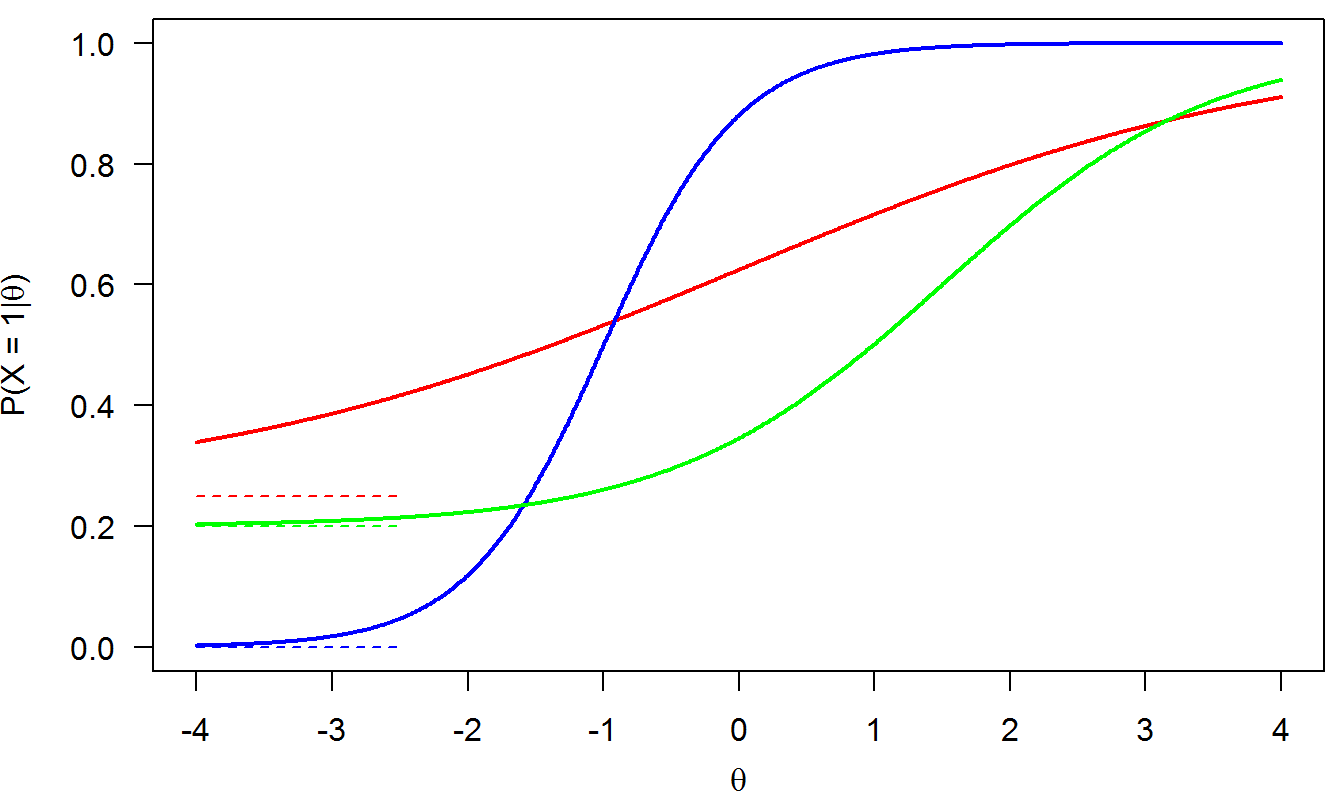
Figure 4.1: 3PLM
Properties of IRFs from the 3PLM:
The 3PLM is a cumulative model: The probability of a correct response is expected to increase with \(\theta\).
The pseudoguessing parameter introduces a lower asymptote to the IRF (symbolized by the dashed horizontal segments on the low-left section of Figure 4.1.
The 3PLM is more flexible than the 2PLM because it allows for different lower asymptotes. However, pseudoguessing parameters are often diffcult to estimate accurately (they are often associated to relatively large SEs). Also, it has been argued that seldom respondents answer to multiple choice items by purely guessing, that is, it is usually the case that one of more distractors are identified. In this case, \(\gamma\) underestimates the real guessing probability involved in the answering process. For these reasons, one should carefully check whether the 3PLM is suitable over and above the 2PLM.
The difficulty parameters \(\delta\) are now slightly differently interpreted. For item \(i\), \(\delta_i\) is the point of the latent trait at which the probability of a correct answer equals \(\frac{\gamma_i + 1}{2}\) (i.e., the midpoint between \(\gamma_i\) and 1). For example, for the green item (\(\delta=1.5\), \(\alpha=1\), \(\gamma=.20\)), we have that (check this using the IRF!)
\[ P(X_i = 1|\theta = 1.5) = \frac{.20+1}{2} = .60. \]
The discrimination parameters are similarly interpreted as in the 2PLM.
The 3PLM has many similarities with the MMH model, however for the 3PLM the IRFs are parametric logistic functions.