IRT (GMMSGE01): Parametric IRT (dichotomous data)
Jorge N. Tendeiro
14 December 2017
1 Main idea
Parametric item response theory (IRT) provides a theoretical framework that allows modeling the relationship
\[\text{item} \longleftrightarrow \text{person}\]
by means of a mathematical function: \[P(X_i = c|\theta_n) = f(\theta_n)\]
\(X_i\) is the random variable denoting the answer to item \(i\), with discrete response categories;
- \(c\) is the observed response:
- If \(X\) is dichotomous, \(c=0,1\). Usually 0 denotes incorrect answers and 1 denotes correct answers.
- If \(X\) is polytomous, \(c=0,1,\ldots,m\) (\(m>1\)).
\(\theta_n=\) \(n^\text{th}\) person’s trait parameter.
This is the item response function (IRF). The IRF is therefore a function relating the latent trait to the probability of answering the item correctly.
In IRT, items and persons are located on the same latent scale. For example, see Figure 1.1 displaying the IRF of a dichotomous item. The item location or difficulty (to be defined shortly) is indicated by the value \(b\) in the \(x\)-axis for which the probability of a correct answer is .50. Thus, values in the \(x\)-axis denote item locations. Moreover, values in the \(x\)-axis can also be interpreted as person latent scores \(\theta\). For example, a person with parameter \(\theta=2\) (i.e., \(\theta > b\)) has probability above .50 of answering this item correctly. Similarly, persons with trait \(\theta < b\) are more likely to answering this item incorrectly.
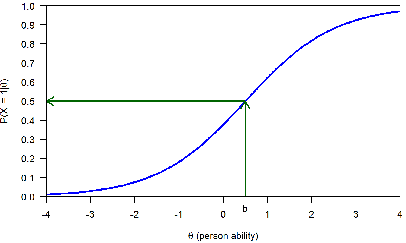
Figure 1.1: Items and persons located on a common scale
The main assumptions of the mainstream parametric IRT models are the following:
The IRF has a mathematically closed form that, when plotted, looks like a smooth S-shaped curve (see Figure 1.1).
Responses to items are independent conditional of \(\theta\). This is known as local independence. In mathematical terms:
\[ P(X_i = 1, X_j = 1| \theta) = P(X_i = 1| \theta)P(X_j = 1| \theta)\]
- Unidimensionality: One latent trait suffices to explain the relationship between the items.
In this lecture we will cover the mostly used IRT models for dichotomous data: The one-, two-, and three-parameter logistic models. We will also talk briefly about model estimation and model fit.