3 The 2PL model (2PLM)
The 2PLM generalizes the 1PLM by adding a new item parameter known as the discrimination parameter. The IRF for item \(i\) is given by
\[\begin{equation} P(X_i=1|\theta) = \frac{\exp[\alpha_i(\theta - \delta_i)]}{1 + \exp[\alpha_i(\theta-\delta_i)]}, \tag{3.1} \end{equation}\]where \(\alpha_i\) is the discrimination parameter for item \(i\). This parameter takes on positive real values, although values larger than, say, 4 or 5 are not common.
Figure 3.1 shows three examples of IRFs under the 2PLM. The difficulties are the same as in Figure 2.1. The discrimination parameters are as follows: \(\alpha = 2\) (blue), \(\alpha = .5\) (red), and \(\alpha = 1\) (green).
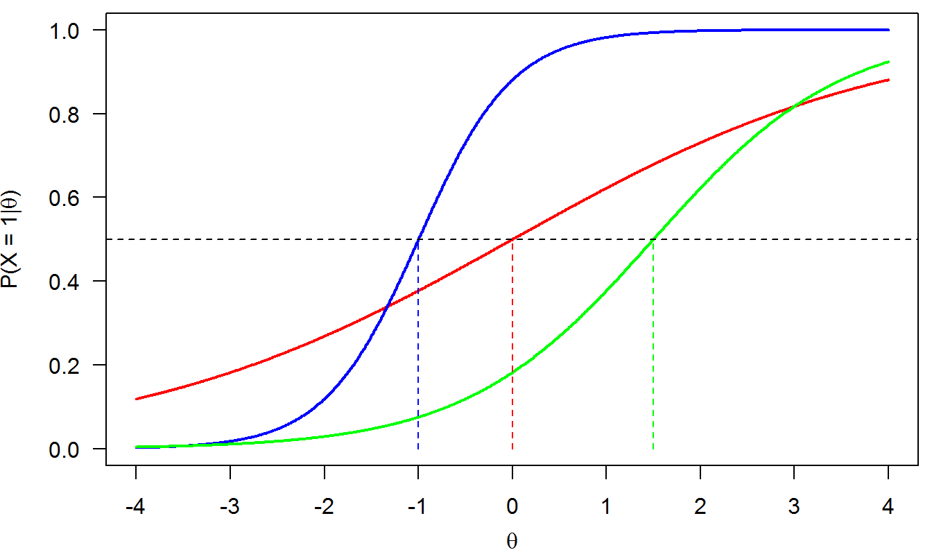
Figure 3.1: 2PLM
Properties of IRFs from the 2PLM:
The 2PLM is also a cumulative model: The probability of a correct response is expected to increase with \(\theta\).
The discrimination parameter determines the steepness of the curve at the difficulty point: The larger \(\alpha\), the steeper the curve. Steeper curves are better to distinguish (discriminate) among persons standing close to each other in this reagion of the latent trait.
The difficulty parameters \(\delta\) are equivalently interpreted as in the 1PLM.
The IRFs may now intersect, as Figure 3.1 shows. So, items may be differently ranked in terms of difficulty for varying levels of \(\theta\).
The 2PLM is more flexible than the 1PLM because it allows items to differ in terms of discrimination. When all items have similar discrimination then the 1PLM is preferred (for parsimony).