5 Model estimation
Two sets of parameters need to be estimated when fitting an IRT model: The item parameters (difficulty, discrimination, pseudoguessing) and the person parameters (\(\theta\)). There are various estimation algorithms available for items (joint maximum likelihood, conditional maximum likelihood, marginal maximum likelihood, and Bayesian MCMC). Given the estimated item parameters, there are then various estimation algorithms for the person parameters (maximum likelihood, MAP, EAP). Here we will only lay out the general principle concerning maximum likelihood estimation for person scoring. So, we will assume that the item parameters are known and explain how the \(\theta\) parameters are then estimated.
5.1 Person scoring
Suppose we have scores of \(N\) persons on \(I\) items collected in an \(N\times I\) data matrix. For person \(s\) (\(s=1,\ldots,N\)) the response pattern is denoted by \(X_s = (u_{s1}, u_{s2}, \ldots, u_{sI})\), where each item score \(u_{si}\) (\(i=1, \ldots, I\)) is either 0 (incorrect answer) or 1 (correct answer). The probability of observing this response pattern under the IRT model of interest (1PLM, 2PLM, or 3PLM) is given by
\[\begin{equation} P(X_s|\theta_s) = \prod_{i=1}^I P_{si}^{u_{si}}(1-P_{si})^{1-u_{si}}, \tag{5.1} \end{equation}\]where \(P_{si} = P(X_i = 1 | \theta_s)\), that is, the probability of person \(s\) providing a correct answer to item \(i\). The explicit formula for \(P_{si}\) depends on the IRT model one wants to fit to the data (Equation (2.1) for the 1PLM, Equation (3.1) for the 2PLM, or Equation (4.1) for the 3PLM). For example, if \(I=4\) and the response pattern is \(X_s = (1, 1, 1, 0)\) then Equation (5.1) is equal to
\[ P(X_s|\theta_s) = P_{s1}P_{s2}P_{s3}(1-P_{s4}). \] We are allowed to multiply the item probabilities across person’s \(s\) response pattern due to the local independence assumption.
Equation (5.1) defines the likelihood function for \(\theta_s\):
\[\begin{equation} L(\theta_s|X_s) = \prod_{i=1}^I P_{si}^{u_{si}}(1-P_{si})^{1-u_{si}}. \tag{5.2} \end{equation}\]With known item parameters, Equation (5.2) is a (rather complex) function of \(\theta_s\) only. MLE tries to finds the value for \(\theta_s\), say \(\widehat{\theta}_s\), that maximizes the likelihood function. That is, \(\widehat{\theta}_s\) is the value that makes it more likely that a person with this latent trait produces a response pattern such as \(X_s = (u_{s1}, u_{s2}, \ldots, u_{sI})\).
Typically it is the natural logarithm of the likelihood function that one maximizes, for numerical reasons (observe that this is allowed because the logarithm function is monotonic). So, the function being maximized is given by
\[\begin{equation} \ln L(\theta_s|X_s) = \sum_{i=1}^I u_{si}\ln(P_{si}) + (1-u_{si})\ln(1-P_{si}). \tag{5.3} \end{equation}\]The algorithm used to estimate \(\theta_s\) is iterative (commonly based on the Newton-Raphson method). The algorithm proceeds as follows:
Specify a starting value for \(\theta_s\), say, \(\theta_s^{(0)}\) (e.g., 0).
Compute the first- and second-order derivatives of the log-likelihood function (Equation (5.3)) at \(\theta_s^{(0)}\), say, \(D1(\theta_s^{(0)})\) and \(D2(\theta_s^{(0)})\). The explicit formulas for these derivatives under the 1PLM, 2PLM, or 3PLM can be found, for example, in Baker and Kim (2000) and Embretson and Reise (2000, for the 1PLM and 2PLM only).
Compute \(\varepsilon_1 = D1(\theta_s^{(0)}) / D2(\theta_s^{(0)})\).
Update \(\theta_s\):
\[\theta_s^{(1)} = \theta_s^{(0)} - \varepsilon_1\].
- Repeat steps 2-4 using the updated \(\theta\) from the last step. Proceed until \(|\varepsilon|\) is smaller than a predefined threshold (e.g., .001) or until a maximum number of iteration steps has been reached (e.g., 100).
This method is expected to converge to the maximum of the (log) likelihood function.
5.2 Information, SE
The standard error (SE) of the estimated person parameter \(\widehat{\theta}_s\) provides a measure of uncertainty of the estimate. The SE is directly related to the so-called item information function. This function indicates what regions of the theta scale are measured more precisely by the item (higher information) and what regions are measured less precisely (lower information).
For a dichotomous item, the item information function is given by (see Baker & Kim, 2004)
\[\begin{equation} Inf_i(\theta) = \left[\alpha_i^2\frac{1-P_i(\theta)}{P_i(\theta)}\right] \left[\frac{P_i(\theta)-\gamma_i}{1-\gamma_i}\right]^2. \tag{5.4} \end{equation}\]This function applies for the 3PLM, the 2PLM (\(\gamma_i=0\)), and the 1PLM (\(\gamma_i=0\), \(\alpha_i=1\)).
The test information function is simply the sum of all item information functions:
\[\begin{equation} TInf(\theta) = \sum_{i=1}^I Inf_i(\theta). \tag{5.5} \end{equation}\]Finally, it can be shown that
\[\begin{equation} SE(\theta) = \frac{1}{\sqrt{TInf(\theta)}}. \tag{5.6} \end{equation}\]5.3 Small example
Let’s focus on a small toy example (Embretson & Reise, 2000). We want to estimate \(\theta\) based on the 2PLM and three items, as shown below:
| Item | Item score | alpha | delta |
|---|---|---|---|
| 1 | 1 | 1.0 | -1.5 |
| 2 | 1 | 1.5 | 0.0 |
| 3 | 0 | 2.0 | 1.5 |
The item response functions look like this (see Equation (3.1)):
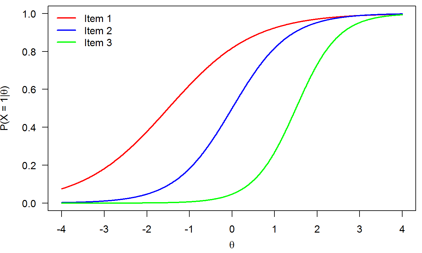
Figure 5.1: IRFs from the toy example
The likelihood function is given by
\[\begin{equation} L(\theta_s|X_s=(1, 1, 0)) = P_{s1}P_{s2}(1-P_{s3}), \tag{5.7} \end{equation}\]where:
\(P_{s1} = \frac{\exp[1.0(\theta - (-1.5))]}{1 + \exp[1.0(\theta-(-1.5))]}\),
\(P_{s2} = \frac{\exp[1.5(\theta - 0.0)]}{1 + \exp[1.5(\theta-0.0)]}\),
and
- \(P_{s3} = \frac{\exp[2.0(\theta - 1.5)]}{1 + \exp[2.0(\theta-1.5)]}\).
The log-likelihood function is given by
\[\begin{equation} \ln L(\theta_s|X_s=(1, 1, 0)) = \ln(P_{s1}) + \ln(P_{s2}) + \ln(1-P_{s3}). \tag{5.8} \end{equation}\]The plot of the likelihood function in Equation (5.7) is displayed in Figure 5.2 (top panel), whereas the log-likelihood function in Equation (5.8) is displayed in Figure 5.2 (bottom panel).
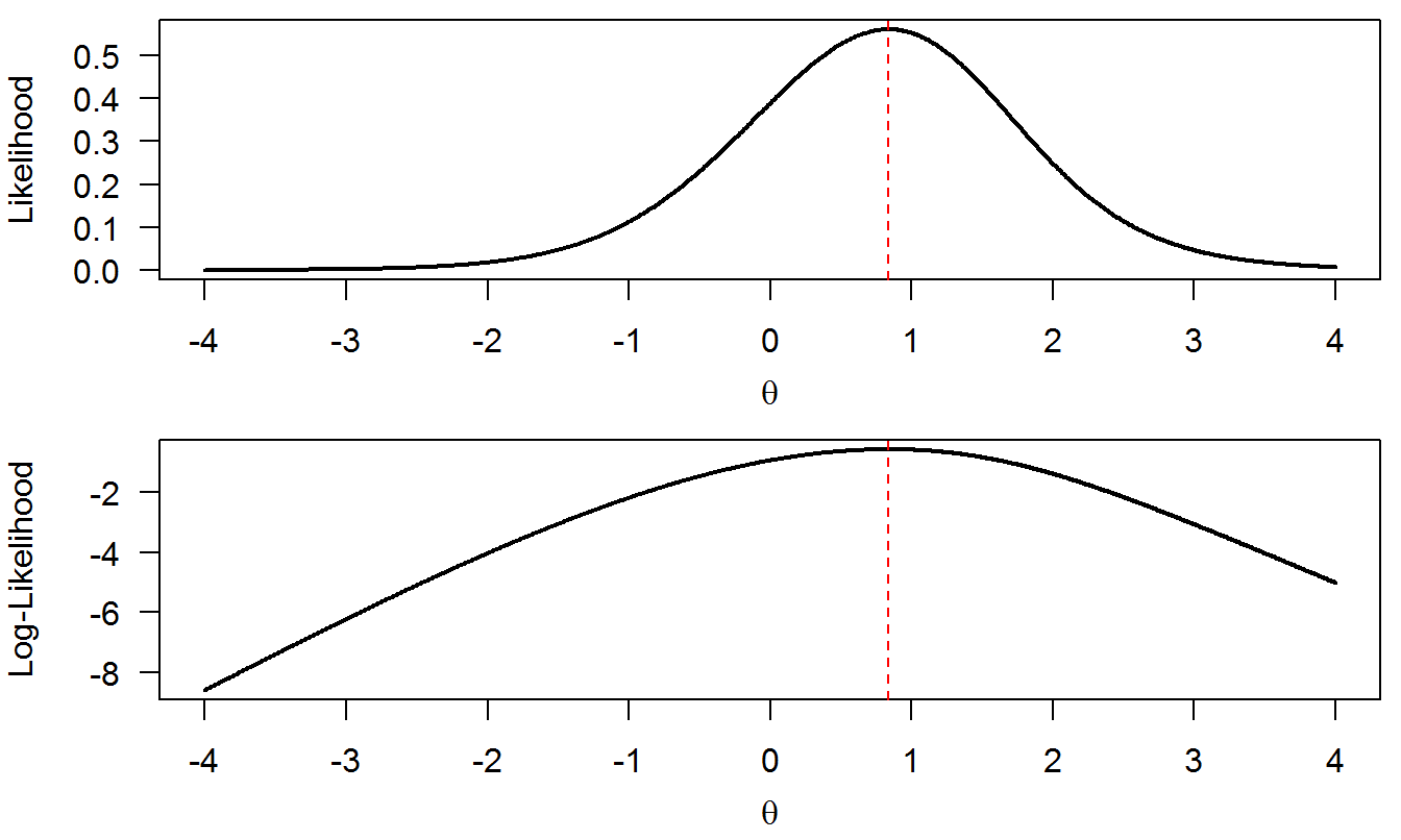
Figure 5.2: Likelihood and log-likelihood functions from the toy example
The MLE for parameter \(\theta_s\) is the value of \(\theta\) that maximizes the likelihood/ log-likelihood function. Observe that the same \(\theta\) value (slightly below 1) maximizes both the likelihood and the likelihood functions simultaneously; this is indicated in both panels by the vertical red dashed line. This is always the case. Again, the log-likelihood is used for numerical convenience.
The seeked value is \(\widehat{\theta}_s=.838\). This value is found by the Newton-Raphson method (initial \(\theta\) value: 0; convergence threshold: .0001; number of steps required: 5).
Next we look at the item and test information functions and the SE of the person parameter estimate. The three item information functions look as follows (see Equation (5.4)):
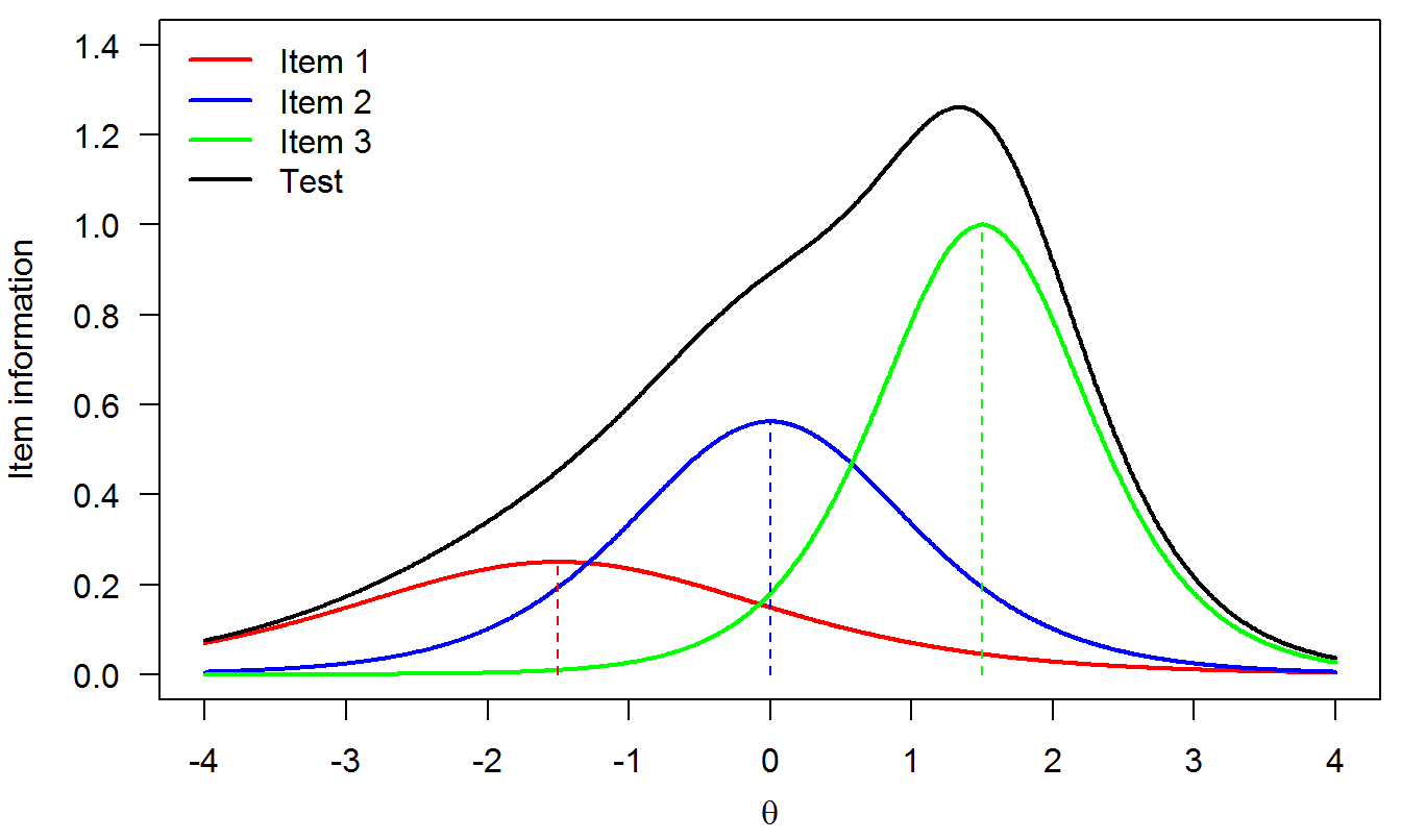
Figure 5.3: Item and test information functions
Two important properties of item information functions are immediately visible:
The item information is maximum at its difficulty level (marked by the vertical dashed lines). This is true for the 1PLM and the 2PLM (not for the 3PLM due to the effect of the pseudoguessing parameter).
Item information increases with the discrimination parameter.
The test information function (Equation (5.5)) is the sum of the three item information functions (black curve in Figure 5.3). It can be seen that this “test” is mostly useful to assess persons with latent ability, say, between 0 and 2 (where the test information function attains high values). This test does not measure persons reliably in the rest of the latent trait because no items were located in these regions.
Finally, the SE conditional on \(\theta\) (Equation (5.6)) is shown in Figure 5.4. Of course, these SE values are unnaceptably large because this toy example is based on three items only. As the number of items increases the measurement precision (and therefore SE) decreases, as expected. That is why a test with more questions is typically more informative than a test with fewer items, all other things being equal. For the person who answered \((1, 1, 0)\) to the three items, we had already seen that \(\widehat{\theta}_s=0.838\). The associated SE is 0.94 (red dashed line).
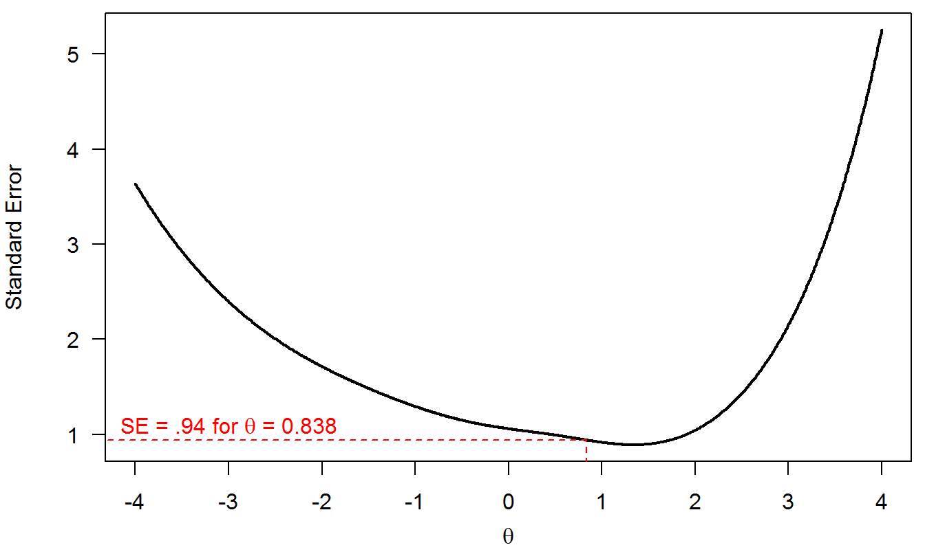
Figure 5.4: SE of measurement
Some properties of the SE:
The test information function (Equation (5.5)), and therefore the SE, does not depend on the particular persons who took the test. This is unlike CTT and its reliability coefficient.
The SE changes with \(\theta\): The test measures persons with more precision (i.e., lower SE) in the latent scale regions with the highest information. This is also unlike CTT, for which the SE is constant for all person scores.
5.4 Model indeterminacy
It should be said that IRT models are typically not identified. That means that there are infinite sets of item and person parameters that lead to the exact same model fit. This is easy to understand by considering the 2PLM. Observe that
\[ P(X=1|\theta) = \frac{\exp[\alpha(\theta-\delta)]}{1+\exp[\alpha(\theta-\delta)]} = \frac{\exp\{\alpha[(\theta+\lambda)-(\delta+\lambda)]\}}{1+\exp\{\alpha[(\theta+\lambda)-(\delta+\lambda)]\}}.\] Visually, this means that we can move all persons and items together left or right on the latent scale by an amount given by \(\lambda\) without affecting the probability of a correct answer. This is a location indeterminacy. There is also a scale indeterminacy: \(\alpha\) can be multiplied by any constant as long as \((\theta+\lambda)\) and \((\delta+\lambda)\) are divided by that same constant.
To solve this problem, model constraints need to be introduced that solve both the location and scale indeterminacies.
5.5 MLE properties
MLE enjoys some good asymptotic (large sample) properties, namely:
Bias: MLEs converge in probability to the true parameter;
Efficiency: MLEs have the smallest mean square error among all consistent estimators;
Residuals are normally distributed.
However:
\(\widehat{\theta}_s\) does not exist for all-0s response patterns (e.g., \((0, 0, 0, 0)\)) or all-1s response patterns (e.g., \((1, 1, 1, 1)\)).
The good properties above hold for large samples only.
The model must be well specified.
5.6 Example
This example is to be found in Embretson and Reise (2000, Chapter 7). The table below shows an example of MLE \(\theta\) estimates based on known item parameters:
Test A: All \(\alpha = 1.5\), and \(\delta = [-2.0,-1.5,-1.0,-0.5,0.0,0.0,0.5, 1.0, 1.5, 2.0]\)
Test B: All \(\delta = 0.0\) and \(\alpha = [1.0, 1.1, 1.2, 1.3, 1.4, 1.5, 1.6, 1.7, 1.8, 1.9]\)
| Person | Resp. pattern | Theta (Test A) | SE (Test A) | Theta (Test B) | SE (Test B) |
|---|---|---|---|---|---|
| 1 | 1111100000 | 0.00 | 0.54 | -0.23 | 0.43 |
| 2 | 0111110000 | 0.00 | 0.54 | -0.13 | 0.43 |
| 3 | 0011111000 | 0.00 | 0.54 | -0.04 | 0.42 |
| 4 | 0001111100 | 0.00 | 0.54 | -0.04 | 0.42 |
| 5 | 0000111110 | 0.00 | 0.54 | 0.13 | 0.43 |
| 6 | 0000011111 | 0.00 | 0.54 | 0.23 | 0.43 |
| 7 | 1110000000 | -0.92 | 0.57 | -0.82 | 0.51 |
| 8 | 0111000000 | -0.92 | 0.57 | -0.74 | 0.50 |
| 9 | 0011100000 | -0.92 | 0.57 | -0.66 | 0.48 |
| 10 | 0001110000 | -0.92 | 0.57 | -0.59 | 0.47 |
| 11 | 0000111000 | -0.92 | 0.57 | -0.53 | 0.46 |
| 12 | 0000011100 | -0.92 | 0.57 | -0.46 | 0.45 |
| 13 | 0000001110 | -0.92 | 0.57 | -0.4 | 0.45 |
| 14 | 0000000111 | -0.92 | 0.57 | -0.34 | 0.44 |
| 15 | 1000000000 | -2.20 | 0.78 | -1.8 | 0.88 |
| 16 | 1100000000 | -1.47 | 0.63 | -1.2 | 0.62 |
| 17 | 1110000000 | -0.92 | 0.57 | -0.82 | 0.51 |
| 18 | 1111000000 | -0.45 | 0.55 | -0.51 | 0.46 |
| 19 | 1111100000 | 0.00 | 0.54 | -0.23 | 0.43 |
| 20 | 1111110000 | 0.45 | 0.55 | 0.04 | 0.42 |
| 21 | 1111111000 | 0.92 | 0.57 | 0.34 | 0.44 |
| 22 | 1111111100 | 1.47 | 0.63 | 0.71 | 0.49 |
| 23 | 1111111110 | 2.20 | 0.78 | 1.28 | 0.65 |
Note that:
For test A, it does not matter which items are answered correctly. Thus ML scoring is insensitive to the consistency of an examinee’s response pattern. This is common to the 1PLM (the number-correct score is a sufficient statistic for \(\theta\)).
The SEs are rather large (small test, only consisting of 10 items).
On test B it is possible to obtain a higher raw score and receive a lower latent trait score (e.g., examinee 18 and examinee 14). This is typical to the 2PLM and the 3PLM.
Examinees who endorse the items with the highest discrimination parameters receive the highest trait scores.