Chapter 3 Week 3 Lab

Homework for Next Week

Fill in all of the answer blocks and coding tasks in this lab notebook.

Complete all tasks in the Homework section (bottom of the Rmd).

Learning Objectives

Learn and apply methods to assess genome assembly quality.

Continuing improving at writing functions.

Explore our data and assess potential issues with quality and contamination.

Start planning some filtering to create and save cleaner genomes for future use.

The majority this lab’s material was developed by your TA, Joel Rodriguez-Medina.

3.0.1 Overview

This week we will work to understand the quality of our genome assemblies, and we will start thinking about issues of contamination. Reminder, an assembly is the set of contigs that were created by combining (assembling) the short sequencing reads into longer stretches. As you are seeing in your data, these assemblies are made of many contigs (sometimes thousands), though only a few of them are very large. We’ll see today that our assemblies are messy, particularly for the smallest contigs. We will work on assessing this quality to plan out a filtering process to create updated contigs for our halophiles of interest. This will allow us to perform genome annotation (the computational process of identifying genes along the genome).

3.0.2 HW 2 (looking over our data)

Brief skim over the google doc to see what everyone found.

3.0.3 Assessing assembly quality in R

3.0.3.1 For local (non RStudio Cloud) users

If you are using RStudio locally (as in, downloaded on your computer and not in RStudio Cloud), there should not be any extra work for you. The only important thing is that your primary strain FASTA files is inside a folder called “data”, and that the “data” folder is in the same folder as this lab 3 Rmd file.

3.0.4 Coding an genome assembly quality analyzer (N50 and L50)

Let’s begin our analysis by writing some more functions in R. But first, let’s load the data. We can work with the example FASTA file, strain1926.fasta. To load the data into R, we’ll use the Biostrings package, which you briefly learned about during the Lab 2 homework. This package allows us to handle the sequence data more easily.

You can learn more about Biostrings by reading the Biostrings manual.

The readDNAStringSet() reads the FASTA format and it converts it into a nicer, (easier-to-work-with) table-like object. The object has 3 columns:

width is the length of the contig
seq is the sequence itself
names is the identifiers or names of each contig.

3.0.4.1 Note: why Biostrings?

R doesn’t play well with long strings. When it tries to print them in the Console, it often crashes. For example, the code

myFasta <- read.table("../data/strain1926.fasta")

myFasta

will make RStudio crash…

So we’re happy we have a DNAStringSet object to work with. Let’s get started.

# loading the assembled genome of strain 1926
strain_1926 <- readDNAStringSet("data/strain1926.fasta")

# see what the object looks like
strain_1926

# see number of contigs, and the width (number of base pairs) for each contig
length(strain_1926)  # number of contigs
width(strain_1926)  # creates a vector with the width/length of each contig

3.0.4.2 Useful Biostrings functions

The width() function retrieves the column with the length of the sequences, and returns it as a vector.

alphabetFrequency() is a function that computes the frequency of each letter in the sequence. There are two important arguments to the function: * baseOnly=TRUE will just use the 4 common bases (A,T,C,G). Any non-base letter gets classified as “other”. * as.prob=TRUE gives the freqeuency as a percentage.

# To get just the sequence for a contig, you can use the double brackets
strain_1926[[1]] # sequence for the first contig

# To get the frequency of bases, you use alphabetFrequency()
alphabetFrequency(strain_1926[[1]])
alphabetFrequency(strain_1926[[1]],baseOnly=TRUE)

# Note that using `as.prob=TRUE` 
alphabetFrequency(strain_1926[[1]],baseOnly=TRUE, as.prob = TRUE)
# is the same as dividing the frequency by the size of the sequence: 
alphabetFrequency(strain_1926[[1]],baseOnly=TRUE)/width(strain_1926)[1]

# size/length/width of contigs
width(strain_1926) # The length of each contig
sum(width(strain_1926)) # The total genome size

These are useful functions. We’ll focus first on the size of each contig. This is critical to the calculation of the values like N50 and L50 that were discussed in the reading. Let’s start with a quick Zoom poll to jog our memories.

For a brief summary here, let’s imagine you’ve ordered all of your contigs from longest to shortest. (Conveniently, this is how our data are organized by default.) We want to know the distribution of our contig lengths. In other words, do we have a few very long contigs that make up most of our total sequence length, or do we have many small contigs that add up to a large fraction of the total? Long contigs will give us more information about where genes are located relative to each othe. And short contigs have a higher chance of being contamination from little bits of foreign DNA that snuck into the process (during culturing, during gDNA extraction, or during sequencing at the MicrobesNG facility). N50 and L50 are both ways to quantify this: they tell us something about relatively how many of our contigs are short or long. As a reminder, these are explained well in the blog post by Elin Videvall.

N50 is a number corresponding to the length of a particular contig. In particular, with our contigs ordered from longest to shortest, it’s the length of the first contig that crosses the halfway point of the total length of all our sequences. So a high number means that a few long contigs make up most of the total length of our sequences. A low number means that many short contigs will make up most of the total length. L50 is a corresponding number for how many contigs it took to reach this halfway point. In fact, if we think of N50 as a specific entry in our vector of widths, L50 is just the position (index) of that N50 value in the vector. These take just a little wrangling to find in R.

# storing our contig lengths as a vector
c_lengths <- width(strain_1926)

total <- sum(c_lengths)

# creating a cumulative sum
c_sum <- cumsum(c_lengths)
plot(c_sum) + abline(a = total/2, b = 0)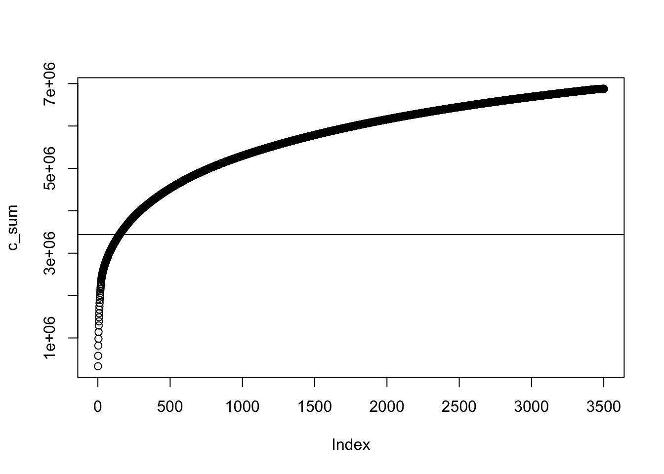

Figure 3.1: figure

## integer(0)

# here we have a function to calculate L50, but 
# the lines are out of order!  Let's fix it.

L_50 <- function(contig_lengths)
{
  contig_ind <- which(contig_sum > sum(contig_lengths)*0.5)
  return(L)
  L <- min(contig_ind)
  contig_sum <- cumsum(contig_lengths)
}


##################################
###       Your code below      
##################################
N_50 <- function(contig_lengths)
{
  # enter your code here
  # hint: you can use other functions inside this
  # function. For example, L_50() might be useful
}


# also, load your own strain into the environment right now as well
# uncomment the next line and replace with the correct numbers for your strain

# strain_XXXX <- readDNAStringSet("data/strainXXXX.fasta")

##################################
##################################

3.0.5 Run the functions with your own genome and update the Google spreadsheet with your N50 and L50.

Google sheet.

3.0.5.1 Questions?

3.0.6 Exploratory Data Analysis.

“Data!data!data!” he cried impatiently. “I can’t make bricks without clay.” – Sherlock Holmes

What does the sequence “GTACAGCAAT” tell you? If you were given a blank piece of paper and told to write up a report on it, what could you write? By itself, perhaps not much. The sequence is 10 characters long; “G”,“C” and “T” appear two times each, while “A” appears twice than that.

But, what if you compare with with another sequence, say “CTTGAAGTGACA”? Now you can say that the two sequences vary in length (one is 10 bp long, the other is 12). The proportion of “A”, “T”,“C”, and “G” is now varied. What would be the best way to present your results? A table? Maybe a graph…what type of graph is the best way to do so?

Much of what we’ll do today is part of what’s called Exploratory Data Analysis and is one of the first steps when analyzing data, especially with large sets such as genomic assemblies. It is a critical step in the overall analysis of data. It can help spotting anomalies (such as outliers, or pieces with low quality); it could also help in the discovery of patterns that can help you generate and test hypothesis about your data.

3.0.7 Exploring GC

How is the percentage of GC content distributed along the contigs? Do all contigs have the same proportion of GC? Are larger contigs richer in GC than smaller contigs?

Using the alphabetFrequency() function we can calculate the GC proportion for the first contig as follows:

# example for only first contig
gc_contig1 <- sum(alphabetFrequency(strain_1926[[1]],baseOnly=TRUE,as.prob = T)[c("G","C")])

# example for all contigs
gc_all_contigs <- rowSums(alphabetFrequency(strain_1926,baseOnly=TRUE,as.prob = T)[,c("G","C")])

3.0.7.1 Coding challenge (15min)

Write a function gc_content() that will take a DNAStringSet and return a vector that is the GC content for each contig.

##################################
###  Your code below           
##################################

gc_content <- function(string_set)
{
  # add your code for the function here.
  # the R example just above this should be useful.
  
  # your input, which we named "string_set", will be a DNAStringSet
}


## below are some extra challenges if you have spare time
## you do not need to complete this as part of the HW/labwork.

# 1) Although it's rare, there will sometimes be a non-zero value
# in the "other" column from alphabetFrequency(). That means that
# adding up the G and C columns isn't quite right. Revisit
# your gc_content() function and adjust it to only calculate GC 
# based on the known A, T, C, and G nucleotides and ignore "others".

# 2) In the Piazza discussion for Week 2, it has come up that
# it's harder to amplify high GC content DNA segments. So one part 
# of Illumina sequencing, the bridge amplification step, might not work as
# well for species or genomic regions with high GC. What are some potential
# consequences of this? For a sample with multiple species, how might 
# this influence the number of contigs you get for each species?


##################################
##################################

We will come back together for discussion and questions, then a 10 min. break.

3.0.8 Data visualization: show, don’t tell.

“Above all else show the data.” – Edward R. Tufte

Meet a new object: the data frame. It’s a type of object in R used to store data tables. It is R’s version of the spreadsheet, but we have many more tools to use with the data. Essentially, each column is a vector, and all columns have the same length. Each column can be a different type of data (some columns could have strings, some could have numbers, some could just have TRUE/FALSE), but within a column all the data must be the same type (can’t mix numbers and text in a single column).

Let’s create a data frame with some data from our strain_1926 data.

# we can start by creating the vectors that will become our columns
# gc content
gc_1926 <- rowSums(alphabetFrequency(strain_1926,baseOnly=TRUE,as.prob = T)[,c("G","C")])

# contig length (we already did this, but let's do it again)
c_lengths_1926 <- width(strain_1926)

# now we define a data.frame
df_1926 <- data.frame(contig_length = c_lengths_1926, gc = gc_1926)

# you can use view() to see it as in a spreadsheet-like format
view(df_1926)

We can use $ to access specific columns:

# we're using head() to avoid printing a super long output
# it's a function that will just show the first few entries in a 
# vector or data.frame

head(df_1926$contig_length)

## [1] 333804 245246 241517 163278 156395 153518

head(df_1926$gc)

## [1] 0.3839768 0.3990198 0.3859190 0.3910018 0.3957416 0.3842611

Remember our original question? “Do all contigs have the same proportion of GC”

head(df_1926)

##   contig_length        gc
## 1        333804 0.3839768
## 2        245246 0.3990198
## 3        241517 0.3859190
## 4        163278 0.3910018
## 5        156395 0.3957416
## 6        153518 0.3842611

We could try looking at the table above, but it only shows the first 6 rows. Data visualization provides an easy way to summarize much larger amounts of information.

We can create plots in R with easy to use built-in functions. Using the plot() function, we just need to tell R which vectors to use for the x- and y-axis values. We can also add a title to the plot with the function argument main.

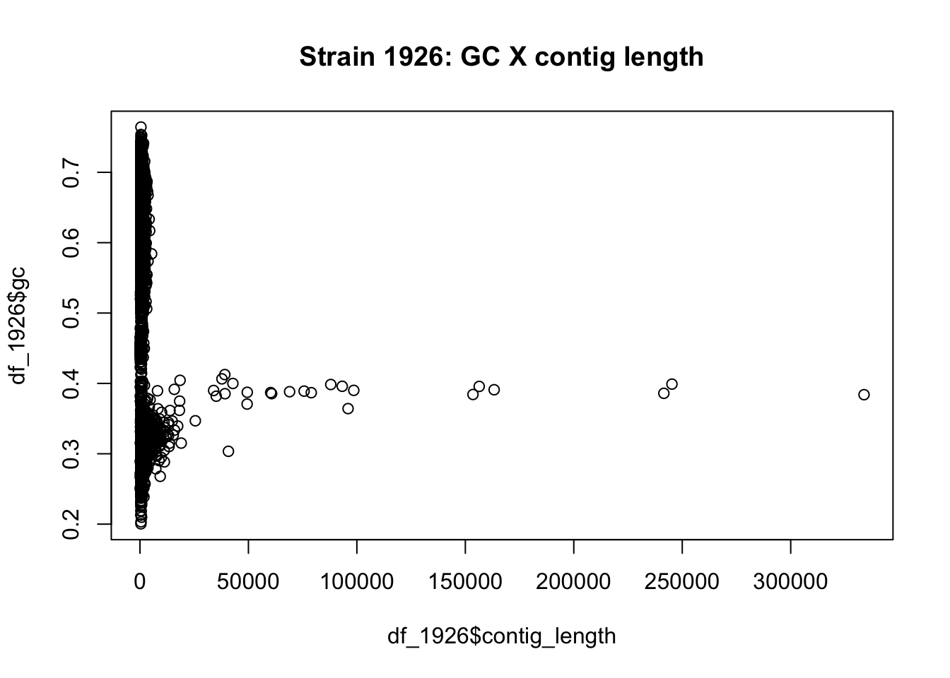
plot(x=df_1926$contig_length, y=df_1926$gc,main="Strain 1926: GC X contig length")

Figure 3.2: figure

Let’s discuss what we see as a class, and relate it to the Week 2 Piazza discussion.

#### Make the same plot for your strain
# You will first need to create a data frame by creating a
# vector for GC and a vector for contig length

##################################
###  Your code below           
##################################

# create a new vector that holds the contig lengths for your strain

# create a new vector with the GC of each contig

# Optional: use data.frame() to create a data frame with a column for each of those
# two vectors (make sure you store this as a new object in your environment)


# create your plot, either from the data frame columns, or
# directly from the vectors
# Make sure you have a title with your strain number


##################################
##################################

3.1 Beautiful evidence.

The base plots in R are a good way to quickly visualize data. The ggplot2 library allows us to have more control over the plotting canvas. Changing the colors, labels and other settings is generally easy.

We can replicate a similar plot to the one above with the following code:

# call the ggplot function and establish the basic canvas settings (X and Y axes)
ggplot(data=df_1926,aes(x=contig_length,y=gc)) +
  geom_point() + # add a geom, i.e. what type of plot to use
  ggtitle("Strain 1926: gc X contig length") # add a title

Figure 3.3: figure

To see exactly what happened at each plotting step, let’s build the plot again, step by step.

df_1926 # The data as is

# calling the ggplot() function and setting the "canvas"
ggplot(data=df_1926,aes(x=contig_length,y=gc))

(#fig:ggplot_StepByStep1)figure

# nothing will display unless you add a "geometry", which
# tells R what kind of visualization to make

ggplot(data=df_1926,aes(x=contig_length,y=gc)) +
  geom_point() # this says we're using points, with x value of each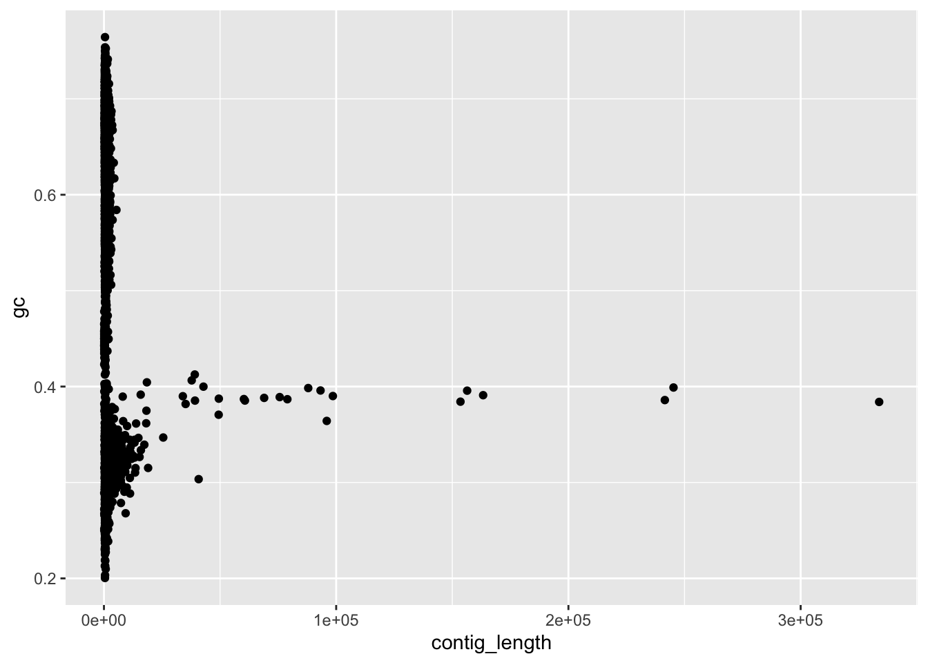

(#fig:ggplot_StepByStep2)figure

# point from the contig_length column and y from the gc column

# the canvas and the geometry are the two key features
# everything else is just a cherry on top

# adding a title
ggplot(data=df_1926,aes(x=contig_length,y=gc)) +
  geom_point() +
  ggtitle("Strain 1926: gc X contig length")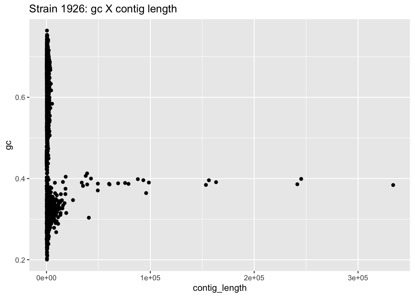

(#fig:ggplot_StepByStep3)figure

# changing the theme for a different shading and axis scheme
ggplot(data=df_1926,aes(x=contig_length,y=gc)) +
  geom_point() +
  ggtitle("Strain 1926: gc X contig length") +
  theme_minimal()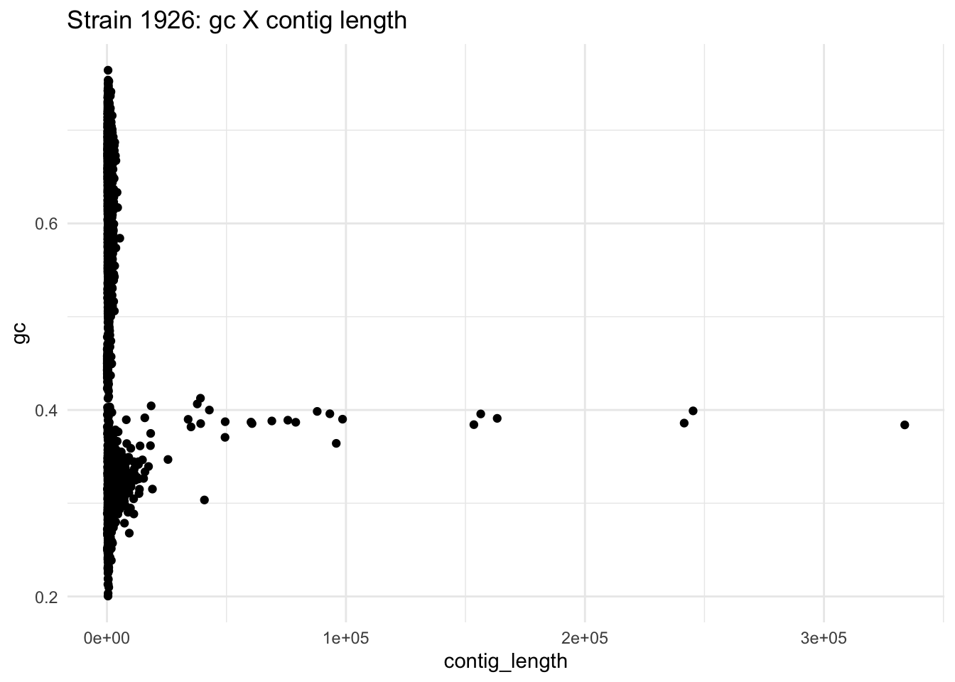

(#fig:ggplot_StepByStep4)figure

3.2 Homework for Week 4, due Wednesday, 4/22, at 10:59pm

Besides the data entry in the google doc, all work should be completed inside of this Rmd file and uploaded to Canvas as a pdf or html file.

3.2.1 Finish up labwork (2 pts)

Make sure that any short responses or coding snippets above have been filled in with your work, and that your other data are entered into the google doc.

3.2.2 Online discussion (part of Week 3 participation points)

Write a follow-up or reply to another student’s follow-up on the Week 3 discussion post on Piazza.

3.2.3 Setting up a RAST account (2 pts)

This will only take a minute. Navigate to the website for an annotation tool called RAST: http://rast.nmpdr.org/?page=Register.

Register, using an email address that you’re comfortable sharing with your instructor. Forward your confirmation email to Dr. Furrow (refurrow@ucdavis.edu).

3.2.4 Readings and response (4 pts)

Next week we are going to try out some research methods from comparative genomics. To get us thinking, part of your homework is to read the first 2 pages (Abstract, Background, and first paragraph of Results), plus Figure 1 on page 3, of this published article. A pdf of the paper is also available on Canvas.

There is some jargon in this paper, so use these reading guide prompts to help keep you focused on the main points.

We haven’t talked much about genes yet in this course. Inside of a gene that codes for a protein (a coding region), successive sets of DNA triplets (called codons) each code for a particular amino acid https://en.wikipedia.org/wiki/DNA_codon_table. The final protein is made up of all of those amino acids attached in sequence, although chaperone proteins combined with chemical and charge-based interactions will cause the protein to fold into some kind of structured, knotted-up bundle as its final functional form. How many different amino acids are there? Do a little online searching to look into the structure of different amino acids. Which ones have negatively charged side chains? Which ones have hydrophobic side chains? (In the presence of water, this will lead the protein to fold to conceal these hydrophobic parts away from the protein’s surface.)
This article mentions the importance of comparing halophiles and non-halophiles of similar GC content. Why is this the case? Think about the codon table you looked at above.
In Figure 1 they performed a cluster analysis. Their data for each strain was the relative usage of each amino acid across all genes in the strain’s genome, and they formed clusters by group together strains with similar patterns of usage. We will go over this in greater detail in Lab 4. The 6 strains at the top of Figure 1 form a cluster distinct from the rest. What do those strains have in common? Are they all in the same Domain (Archaea vs. Bacteria)?
Which amino acids showed patterns specific to Halophiles? What features do these amino acids have in common?
The analysis presented in Figure 1 used both halophiles and evolutionarily related non-halophilic microbes. Why did they include the non-halophiles as well? Did the clusters of amino acid usage they found correspond more to relatedness or to environment (halophile vs. non-halophile)? Any exceptions? (Remember than any bacteria should be more closely related to other bacteria than it is to any archaea, and vice-versa as well.)

3.2.4.1 Your responses (2-3 sentences each)

Q1.

Q2.

Q3.

Q4.

Q5.

3.2.5 Data Exploration (2 points total)

Follow the tutorial for ggplots2 in http://r-statistics.co/Complete-Ggplot2-Tutorial-Part1-With-R-Code.html

Make a ggplot of GC content versus contig length using your genome.

Color the points by the contig size.

Plot the logarithm of the contig length of the raw values.

Change the theme of the plot.

In addition, start thinking about how you might want to filter these data to remove some of the contamination. For example, would you want to eliminate small contigs? Eliminate contigs above or below certain GC content thresholds? If you have two or more groups of long contigs that have different GC content, your best bet is to focus on the highest GC strain. That is most likely to be a halophile and not a skin bacterium (many of which have very low GC, around 30-35%).

Part of Lab 4 will have you filtering your data and saving a new FASTA file, to upload to RAST for annotation. We want to finish that during Lab 4, which is why we are thinking about it now.

##############################
###    Your code below     
##############################

# enter the code for your plotting (and loading your data) here


##############################
##############################

3.3 Code Appendix

This includes all of the inline code you wrote in the coding sections while you were exploring in this week’s lab. You don’t need to write anything – it will automatically fill itself in.

##################################
###  Your code below           
##################################

# create a vector named dog, consisting of the values 5, 7, 9, and 126.3
# remember to wrap the values in the c() function


# use the function mean() to calculate the mean of the vector dog


# use the command ?mean to see R's documentation of the function.
# ? before a function name pulls a useful help file.
# mean() has some extra arguments that you can use. 
# what can you do by setting a trim argument?


# below is a string stored as the object bird
# use strsplit() and table() to count the number of occurrences of the letter r
bird <- "chirp_chirp_i_am_a_bird_chirp"


###
# extra things to play with, time permitting
# check out the help file for strsplit()


# we used the argument split="" to split every character apart.
# try using strsplit() with split="_" on the variable bird.


# what is your output?  (use the # symbol at the start of the line
# to write your response as a comment, otherwise
# R will get confused when you create your final document)



# Can you imagine any scenarios where this might be useful?



##################################
##################################
# Following the approach above, find the percent identity 
# for these two sequences
seq1 <- "CCTAACGTCAGCAGATCAAACGCCGATTC"
seq2 <- "CCGAAGGACTAGCTAGCTAGCGCGGATTG"

##################################
###  Your code below           
##################################



# After calculating it, what do you think? Are these sequences similar?
# We'll gradually get more and more context for this as the course goes on.

##################################
##################################
lab1_hw_reads <- c("GTTATCTAAGACCCATCTTCTCACTGGTCACTCACTCCACTGGCATATTC",
                   "CGAATCTTTTTGTTGTTCGAGAGGCCTGTGACACCCCTGGGTTATCTAAG",
                   "TGGCATATTCGTCAAACAGTTCTGATGCCTGATACAACTGACAAATCTCA")

##################################
###  Your code below           
##################################

# Make sure you include lots of comments!
# Before each of line code where you're doing someting new,
# use # to add a comment to explain what you're doing.

# Remember to create the string named genome and also to 
# calculate GC content.




##################################
##################################

# Use this space to write the code for assembling the mystery sequences
# Assemble mystery2, 3, 4, 5, 6, and 7, and store them as
# a2, a3, a4, a5, a6, a7

##################################
###  Your code below           
##################################

# example for mystery2
a2 <- assemble(mystery2, min_overlap = 5)



##################################
##################################

# Here you have a pre-written function to calculate GC content.
# But, the lines of code ARE IN THE WRONG ORDER!
# Read it over, move the code into the right order,
# and add comments to explain each step.

##################################
###  Your code below           
##################################

count_gc <- function(assembly)
{
    GC <- C_total + G_total
    
    C_total <- sum(assembly_vec == "C")
    
    assembly_vec <- unlist(strsplit(assembly, split = ""))
    
    G_total <- sum(assembly_vec == "G")
    
    return(GC)
}


# When that's complete, use the code from count_gc, 
# but add a few lines so that you return the fraction
# of all nucleotides that are GC, not the total count
# I.e. it should be a number between 0 and 1.

fraction_gc <- function(assembly)
{
    
}

# VALIDATION
# your answer for fraction_gc(a1) should be 0.47 (rounded)
# your answer for fraction_gc(a2) should be 0.59 (rounded)


##################################
##################################
##################################
###  Your code below           
##################################
# use this space to load your FASTA file and get the data requested above.

# template for loading your data as a DNAStringSet
# you'll need to edit the filename to match the FASTA file for
# your strain
my_strain <- readDNAStringSet("data/ENTER_YOUR_STRAIN.fasta")

# for the example (strain 1926), we used the command
# strain_1926 <- readDNAStringSet("data/strain1926.fasta")
# we commented the line above so it won't automatically run






##################################
##################################
# storing our contig lengths as a vector
c_lengths <- width(strain_1926)

total <- sum(c_lengths)

# creating a cumulative sum
c_sum <- cumsum(c_lengths)
plot(c_sum) + abline(a = total/2, b = 0)

# here we have a function to calculate L50, but 
# the lines are out of order!  Let's fix it.

L_50 <- function(contig_lengths)
{
  contig_ind <- which(contig_sum > sum(contig_lengths)*0.5)
  return(L)
  L <- min(contig_ind)
  contig_sum <- cumsum(contig_lengths)
}


##################################
###       Your code below      
##################################
N_50 <- function(contig_lengths)
{
  # enter your code here
  # hint: you can use other functions inside this
  # function. For example, L_50() might be useful
}


# also, load your own strain into the environment right now as well
# uncomment the next line and replace with the correct numbers for your strain

# strain_XXXX <- readDNAStringSet("data/strainXXXX.fasta")

##################################
##################################

##################################
###  Your code below           
##################################

gc_content <- function(string_set)
{
  # add your code for the function here.
  # the R example just above this should be useful.
  
  # your input, which we named "string_set", will be a DNAStringSet
}


## below are some extra challenges if you have spare time
## you do not need to complete this as part of the HW/labwork.

# 1) Although it's rare, there will sometimes be a non-zero value
# in the "other" column from alphabetFrequency(). That means that
# adding up the G and C columns isn't quite right. Revisit
# your gc_content() function and adjust it to only calculate GC 
# based on the known A, T, C, and G nucleotides and ignore "others".

# 2) In the Piazza discussion for Week 2, it has come up that
# it's harder to amplify high GC content DNA segments. So one part 
# of Illumina sequencing, the bridge amplification step, might not work as
# well for species or genomic regions with high GC. What are some potential
# consequences of this? For a sample with multiple species, how might 
# this influence the number of contigs you get for each species?


##################################
##################################
#### Make the same plot for your strain
# You will first need to create a data frame by creating a
# vector for GC and a vector for contig length

##################################
###  Your code below           
##################################

# create a new vector that holds the contig lengths for your strain

# create a new vector with the GC of each contig

# Optional: use data.frame() to create a data frame with a column for each of those
# two vectors (make sure you store this as a new object in your environment)


# create your plot, either from the data frame columns, or
# directly from the vectors
# Make sure you have a title with your strain number


##################################
##################################

##############################
###    Your code below     
##############################

# enter the code for your plotting (and loading your data) here


##############################
##############################

##################################
###  Your code below           ###
##################################

# These tasks are all working with strain 1926

# 1) create a new DNAStringSet called strain_1926_f5000
# that has only contigs of length >= 5000


# 2) create a new data frame called strain_1926_gc_narrow
# that has only contigs of length >= 2000 and gc content < 0.5



##################################
##################################
# Our comments below are reminders of the key steps

##########################
### Your work below    ###
##########################

# Load your data and create a data frame with contig length and gc content
# e.g. strain_XXXX <- readDNAStringSet("data/strainXXXX.fasta")
# df_XXXX <- data.frame(contig_lengths = width(strain_XXXX),gc = gc_content(strain_XXXX))



# Plot the data and look for quality issues
# e.g. ggplot(data = df_xxxx, aes(x = contig_lengths, y = gc)) +
#  geom_point() + 
#  scale_x_log10()



# Use logical comparisons like >,<,>=, etc. combined with &
# to get a TRUE/FALSE vector of the entries you want to keep



# Use that vector to select only certain entries from your 
# DNAStringSet



# Save your new DNAStringSet as a fasta file with the following naming 
# convention: strainXXXX_clean.fasta (replace XXXX with your strain number)



##########################
##########################
# Your task, build the same tree using the infB gene.
# then build a tree combining data from both genes.

##################################
###  Your code below           ###
##################################

# building a tree from infB
# first create a distance matrix. You should
# only need to make a small change to the code above.


# then, use that distance matrix with hclust()


# finally, plot the results



##################################
##################################

##################################
###    Your work below         ###
##################################





##################################
##################################
# we are back to our old friend the DNAStringSet

# let's focus just on the second contig (for arbitrary reasons)
# we can select it with the double brackets
s26_2 <- s26[[2]]

# now s26_1 is in our environment as a single DNAString
# let's use our gc_content_single() function to get the overall GC content
gc26_2 <- gc_content_single(s26_2)

# it's 0.39

# as a quick example, let's get the GC content for just the first 500 bp
# all we have to do is use square brackets to select the base pairs from 
# position 1 up to 500.
gc_content_single(s26_2[1:500])

## live-coding will be written in this chunk