Chapter 7 Marketing
7.1 Optimal Product Mix
At first glance, price optimization may seem complex. But careful review and reflection reveals the concept, and the math behind it, are not as complex as they may first appear. Generally, the higher the price, the lower the volume, all else being equal (which it rarely is). Here I walk through a couple of examples of price optimization for a single, unconstrained offering, and two products under a constrained system.
Basic Price Optimization - Unconstrained, Single Product
Example 1: Acme is looking to set the price of its anvils for the current period. Assume the company’s unit production cost c is a constant $675 per unit and the demand for the current period is governed by the linear price-response function
d(p)=(209000-130p)
Re(polyroot(c(209000,-130)))[1] 1607.692
This means that the demand will be 209,000-130p for prices between 0 and 1,608 (209000/130) and that the demand will be 0 for prices over $1,608. In this example, d’(p)=-130.
Applying an unconstrained model, defined by the equation d(p)=-d’(p)(p-c), solve for the optimal price p.
209000-130p=130(p-675)
or after some algebra,
296750=260p*
p*=$1,141
Alternatively in R
f <- function(x)  ((130+130)*(x)-((130*675)+209000))
uniroot(f, lower=0, upper=10000)$root
[1] 1141.346
At the optimal price of $1,141, total sales will be 209,000-130(1,141) = 60,670 units, total revenue will be 60,670 * $1,141 = $69,224,470, and total contribution will be 60,670($1,141 - $675), or $28,272,220.
A question that often arises is how do we determine the price-response function. Ideally, market research will provide direction, testing for volume indicators from customers at different price points. Unfortunately, this is not always possible and research is expensive and may take months to complete. In absence of research, a price-response function may be derived using historical data. A basic approach is to develop a linear model as described previously, predicting price against volume using historical data. Take caution to remove obvious outliers and if necessary transform variables. An in-depth discussion of the statistics involved is beyond the scope here, but the equation of the line (y = mx + b), with price being on the y axis is in economic terms, similar to though not precisely, the demand curve, or in our case, the price-response function. Some economic literature applies an inverted demand curve which is simply a linear equation with volume on the y axis and price on the x axis. An obvious problem with the model above is that it fails to consider other products in the market and the reality that supply is limited. In the next example, we address both issues.
Price Optimization for Two Products under Constrained Supply
Example 2: Suppose Acme is now looking to optimize prices for two products (perhaps anvils and dehydrated boulders) simultaneously and is supply constrained to 60,000 units per period. Let’s call the first item, product B and the second item product C. Product B is of better quality than product C and Coyote appears willing to pay more for it. We want to find just how much more they are willing to pay. Cost, c, is the same for both products at $675/unit.
Our objective is to find the optimal price for both product B and product C simultaneously under constrained supply.
We determine the price-response curves to be:
Anvils (C): dc(pc)=(110,000-61pc)
Dehydrated Boulders (B): db(pb)=30,000-16pb)
The aggregate demand curve is: d(p)=(110,000-61p)+(30,000-16p)=140,000-77p. This means that the demand for Anvils and Dehydrated Boulders will be 140,000-77p for prices between $0 and $1,818 and that demand will be 0 for prices over $1,818. For comparison, we first apply an unconstrained model, defined by the equation d(p)=-d’(p)(p-c), and solve for the optimal price p.
d’(p)=-77
140000-77p=77(p-675)
Applying algebra, gives us
p*= $1,247
or in R:
f <- function(x)  ((77+77)*(x)-((77*675)+140000))
p <- uniroot(f, lower=0, upper=10000)$root
r <- p*60000
p
[1] 1246.591
r[1] 74795455
Thus, the optimal price for both products is 1,247. At this price, Acme will sell exactly it’s capacity of 60,000 units, grossing 74,820,000.
Now, we compare differential pricing based on our assumption that the company can charge more for it’s Dehydrated Boulders than for it’s Anvils. Finding the optimal price for each product requires solving the constrained optimization problem.
maximize pc(110000-61pc)+pb(30000-16pb)
subject to pc(110000-61pc)+pb(30000-16pb)<=60,000
When supply is unconstrained, marginal revenues should all be set to the marginal cost.
When supply is unconstrained, marginal revenues should still be equated, but they need to be set so that the supply constraint is satisfied.
The marginal revenue is (2pc-(110000/61)) for Anvils, and (2pb-(30000/16)) for Dehydrated Boulders.
Equating the two marginal revenues 2pc-1803=2pb-1875 gives pb=pc+36. In other words, the price for Dehydrated Boulders will be $36/unit higher than the price for Anvils.
The other condition that must be satisifed is that the total demand for both products must be equal to capacity; that is (110,000-61pc)+(30,000-16pb)=60,0000. Solving both conditions simultaneously gives pc=1039 and pb=1074. At these prices, Acme will sell 46623 units of Anvils and 12802 units of Dehyrdated Boulders, thus selling at full capacity of 59426 units. Revenue generated will be 62200656, and total contribution will be $22087951.
With the basics understood, let’s apply this approach to multiple products using R.
f <- function(x)  ((77+77)*(x)-((77*675)+140000))
p <- uniroot(f, lower=0, upper=10000)$root
r <- p*60000
d <- (-(110000/61)+(30000/16))/2

f <- function(x)  ((110000 - (61*(x))) + (30000 - (16*(x)))-60000)
p1 <- uniroot(f, lower=0, upper=10000)$root
p2 <- p1 + d
q1 <- 110000-61*p1
q2 <- 30000-16*p2
total_rev <- (p1*q1)+(p2*q2)
total_cost <- (675*(q1+q2))
total_cont <- total_rev - total_cost
## Warning: package 'dplyr' was built under R version 3.4.2##
## Attaching package: 'dplyr'## The following objects are masked from 'package:stats':
##
## filter, lag## The following objects are masked from 'package:base':
##
## intersect, setdiff, setequal, union## Warning: package 'kableExtra' was built under R version 3.4.4| Measure | Anvils | Dehydrated Boulders | Total |
|---|---|---|---|
| Price | 1039 | 1075 | 1047 |
| Cost | -675 | -675 | -675 |
| Units | 46623 | 12803 | 59426 |
| Contribution | 16969093 | 5118858 | 22087951 |
7.2 Pricing with Subjective Demand
Sometimes you may not be able to accurately calculate price elasticity of demand for a product. In other situations, you may belive the linear or power demand curve is not relevant. In these situations, one way to determine a product’s demand curve is to identify the lowest price and the highest price that seem reasonable (perhaps using like products). You can then estimate the product’s demand midway between the high and low prices. Given these three points (High, Low, Mid), you can use R to fit a quadtratic demand curve with the following equation:
\[Demand = a(price)^2+b(price)+c\] For any three specified points on the demand curve, values a,b,c exist that will make the equation exactly fit the three specified points. Because the equation fits the three points on the demand curve, it seems reasonable to believe that the equation will give an accurate represenation of demand at the other prices. You can then use the equation and R to determine the maximum profit given by the formula:
\[formula=(price-unit cost)* demand\] Let’s walk through an example of how this works. Acme would like to launch a new glue stick, targeted to the Coyote chasing RoadRunner market. Acme pays 0.90 for each unit it orders. Acme is considering charging from 1.50 to 2.50 for a glue stick unit. Acme thinks that at a price of 1.50 it will sell 60 units per week. At a price of 2.00, Acme thinks it will sell 51 units per week, and at a price of 2.50, 20 units per week. What price should Acme charge for its glue stick?
p <- c(1.0, 1.25, 1.5, 2, 2.5, 3.0)
q <- c(80, 65, 60, 51, 20, 5)

df <- as.data.frame(cbind(p,q))

plot(p ~ q, df)

library(ggplot2)
## Warning: package 'ggplot2' was built under R version 3.4.3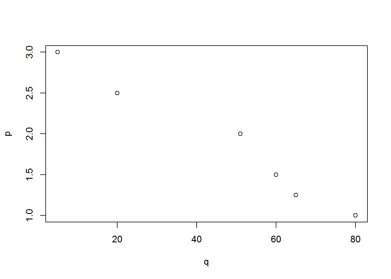
ggplot(df, aes(p,q)) + geom_point() + geom_smooth()## `geom_smooth()` using method = 'loess'## Warning in simpleLoess(y, x, w, span, degree = degree, parametric =
## parametric, : pseudoinverse used at 1.5## Warning in simpleLoess(y, x, w, span, degree = degree, parametric =
## parametric, : neighborhood radius 0.5## Warning in simpleLoess(y, x, w, span, degree = degree, parametric =
## parametric, : reciprocal condition number 0## Warning in predLoess(object$y, object$x, newx = if
## (is.null(newdata)) object$x else if (is.data.frame(newdata))
## as.matrix(model.frame(delete.response(terms(object)), : pseudoinverse used
## at 1.5## Warning in predLoess(object$y, object$x, newx = if
## (is.null(newdata)) object$x else if (is.data.frame(newdata))
## as.matrix(model.frame(delete.response(terms(object)), : neighborhood radius
## 0.5## Warning in predLoess(object$y, object$x, newx = if
## (is.null(newdata)) object$x else if (is.data.frame(newdata))
## as.matrix(model.frame(delete.response(terms(object)), : reciprocal
## condition number 0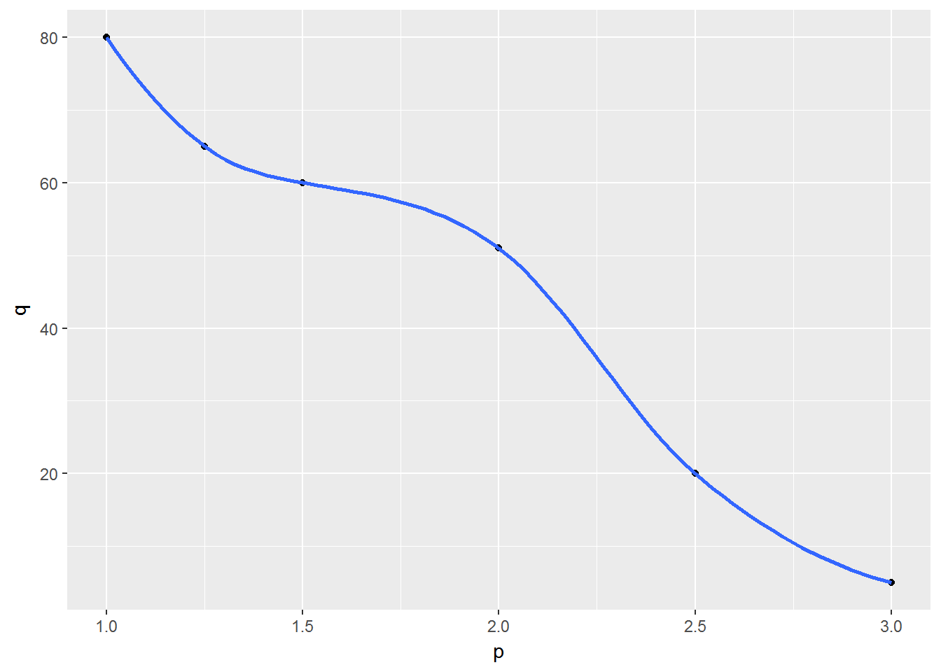
7.3 Determining Customer Value
Acme is struggling to understand its customers and if a specific customer is relevant to its organization. As a Marketing Analyst at Acme, your manager has stated the following objectives:
Objectives:
We want to know how much value a customer is generating for the organization.
We want to know how the generated value is going to evolve.
We want to segment customers based on value.
Why? To perform specific actions for different customer groups
Here, we will cover the techniques used to solve the business problem and respond to the objectives.
We have many options to understand customer’s value. One of the most relevant is CLV. CLV is the acronym of Customer Lifetime Value. CLV is a prediction of all the value a business will derive from their entire relationship with a customer. There is a tough part in this definition: how to estimate future customer interactions.
The calculation of CLV can be based on:
ARPU/ARPA (Historic CLV)
RFM (only applicable to the next period)
CLV Formula (historic CLV)
Probability/Econometrics/ Persistence Models/Machine Learning/Growth and dissemination models such as: Moving Averages, Regressions, Bayesian Inference, Pareto/NBD (Negative Binomial Distribution)
The value generated by all our customers is called Customer Equity and is used to evaluate companies (with no significant income yet).
Main Concepts
There are many factors that affect customer’s value and must be considered in the CLV calculation:
Cash flow: the net present value of the income generated by the customer to the organization throughout their relationship with the organization
Lifecycle: the duration of the relationship with the organization
Maintenance costs: associated costs to ensure that the flow of revenue per customer is achieved Risk costs: risk associated with a client
Acquisition costs: costs and effort required to acquire a new customer.
Retention costs: costs and effort required to retain a new customer.
Recommendation value: impact of the recommendations of a customer in its sphere of influence on company revenue
Segmentation improvements: value of customer information in improving customer segmentation models
CLV Formula
\[ CLV = \sum^{T}{n=0} \frac{(p{t}-c_{t})r_t}{(1+i)^t} - AC \]
where
\(p_t\) = price paid by the customer in time \(t\),
\(c_t\) = direct costs for customer service in time \(t\)
\(i\) = discount rate or cost of money for the firm,
\(r_t\) = probability that the client returns to buy or is alive in time \(t\),
\(AC\) = acquisition cost, and
\(T\) = time horizon to estimate \(CLV\).
Final consideration
Generally we will have a dataset for each of the concepts of the formula
We’ll have to estimate the rest
Therefore, it is important to remember that:
Our ability to predict the future is limited by the fact that to some extent is contained in the past.
- What mathematically means we are under some continuity conditions (or the hyphotesis are true)
Implementation Process
Discuss whether CLV fits as a metric in our business
Identification and understanding of sources and metadata
Extract, transform, clean and load data
Choose CLV method
Analyze results and adjust parameters
Present and explain the results
Benefits
This technique provides the following benefits:
Ability to create business objectives
Better understanding of customers
Having a common numerical analysis criteria
Ability to have an alert system
Improved management of the sales force
Use cases
Create market strategies based on CLV
Customer segmentation based on CLV
Forecasting and customer evolution per segment
Create different communication, services and loyalty programs based on CLV
Awake “non-active” customers
Estimated the value of a company (startup, in the context of acquisition)
How to implement CLV using R
ARPU/ARPA as CLV aproximation
Average Revenue per User (ARPU) and Average Revenue per Account (ARPA) can be used to calculate historical CLV. Process:
calculate the average revenue per customer per month (total revenue ? number of months since the customer joined) add them up
and then multiply by 12 or 24 to get a one- or two-year CLV.
| Customer | Purchase_Date | Value |
|---|---|---|
| Sylvester | 1/1/2007 | 150 |
| Sylvester | 5/15/2007 | 50 |
| Sylvester | 6/15/2007 | 100 |
| Tweety | 5/1/2007 | 45 |
| Tweety | 6/15/2007 | 75 |
| Tweety | 6/30/2007 | 100 |
Suppose today is July 1, 2007. Average monthly revenue from Sylvester is \((150 + 50 + 100)/6 = 50\)
and average monthly revenue from Tweety is \((45 + 75 + 100)/2 = 110\).
Adding these two numbers gives you an average monthly revenue per customer of $160/2 = $80. To find a 12-month or 24-month CLV, multiply that number by 12 or 24.
The benefit of an ARPU approach is that it is simple to calculate, but it does not take into account changes in your customers’ behaviors
Let’s understand the CLV formula by taking a closer look at the Sales data set, a sample of 71,962 transcations, aggregated monthly dating back to January 2002.
# Load data into a dataframe
df <- read.csv('https://raw.githubusercontent.com/jmonroe252/RforBusiness/master/sales_hist.csv', stringsAsFactors = FALSE)

head(df)| Date | Customer_ID | Customer | Product | Value | Units |
|---|---|---|---|---|---|
| 12/1/2017 | 68 | Yosemite Sam | Iron Bird Seed | 304217.0 | 283 |
| 12/1/2017 | 68 | Yosemite Sam | Earthquake Pills | 270966.0 | 299 |
| 12/1/2017 | 68 | Yosemite Sam | Hi-Speed Tonic | 688150.0 | 609 |
| 12/1/2017 | 68 | Yosemite Sam | Dehydrated Boulder | 334638.7 | 235 |
| 12/1/2017 | 68 | Yosemite Sam | Invisible Paint | 292643.3 | 254 |
| 12/1/2017 | 68 | Yosemite Sam | Anvil | 729439.0 | 579 |
Let’s organize our data a bit, and plot how customers are evolving from a dollar value perspective.
df <- read.csv('https://raw.githubusercontent.com/jmonroe252/RforBusiness/master/sales_hist.csv', stringsAsFactors = FALSE)

# Let's practice some data clean-up
df$Date <- as.Date(df$Date, "%m/%d/%Y")

# Aggregate by year
short.date = strftime(df$Date, "%Y")
aggdata = aggregate(df$Value ~ short.date, FUN = sum, na.rm=TRUE)
aggdata <- plyr::rename(aggdata, c("df$Value" = "Value"))

# Graph: how the number of customers is evolving
ggplot(aggdata, aes(x = short.date, y = Value, group=1)) +
  geom_line() + ggtitle("Order Value") +
  ylab("$Value") + xlab("") +
  theme(plot.title = element_text(color="#666666", face="bold", size=20, hjust=0)) +
  theme(axis.title = element_text(color="#666666", face="bold", size=14)) +
  theme(axis.text.x = element_text(angle = 90, hjust = 1))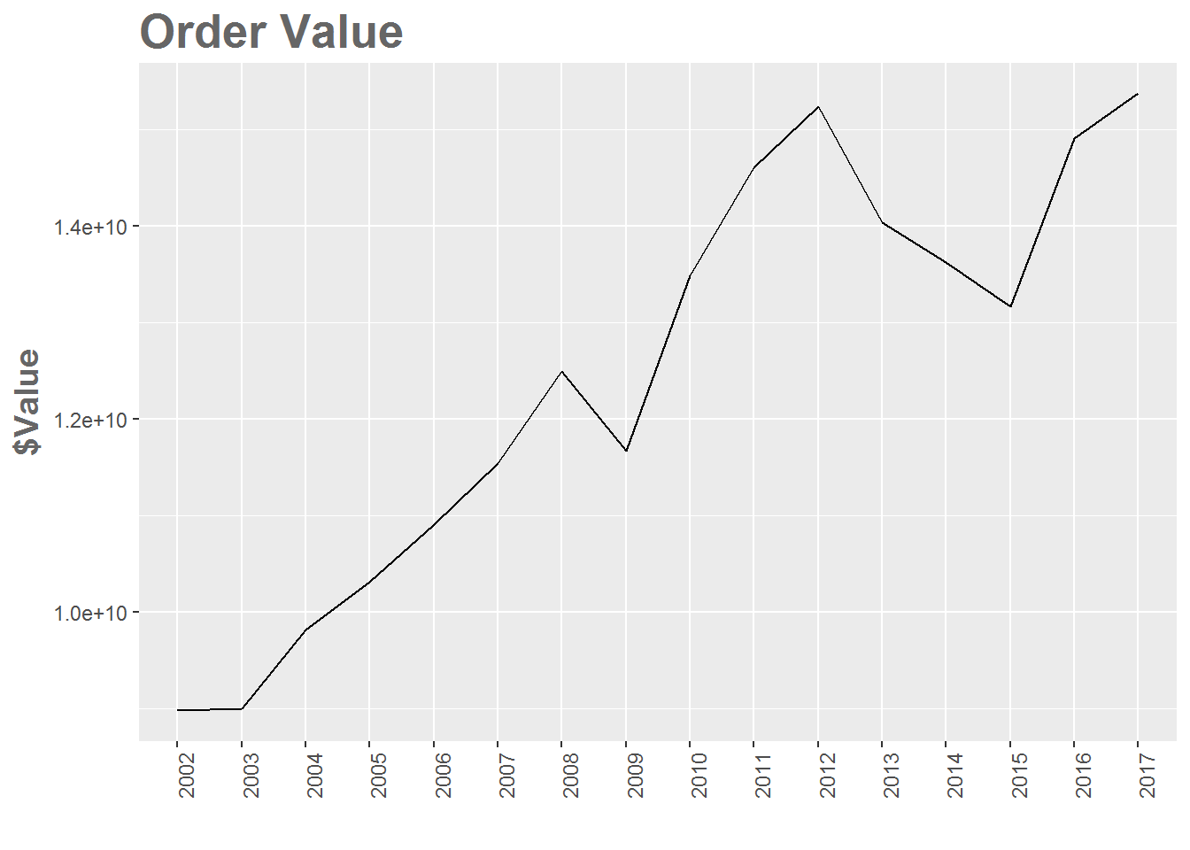
Total sales were generally increasing until 2012 (even Acme was not immune to the Great Recession), declined through 2015, but back to increasing in 2016 and 2017.
Let’s now compute additional key marketing indicators:
recency: time since last purchase (months)
frequency: number of purchase transactions
year of purchase
avg_amount: average amount spent
library(dplyr)
#### Create recency variable

df <- read.csv('https://raw.githubusercontent.com/jmonroe252/RforBusiness/master/sales_hist.csv', stringsAsFactors = FALSE)

#### Let's practice some data clean-up
df$Date <- as.Date(df$Date, "%m/%d/%Y")

df$date_of_purchase = as.Date(df$Date, "%Y-%m-%d")
df$year_of_purchase = as.numeric(format(df$date_of_purchase, "%Y"))
df$days_since       = as.numeric(difftime(time1 = "2017-12-01",
                                            time2 = df$date_of_purchase,
                                            units = "days"))

#### Customer database as at end of 2017 grouped by Customer_ID with remaining market indicators computed

df_17 <- df %>%
        group_by(Customer_ID) %>%
        summarise(recency = min(days_since),
                  frequency = n(),
                  first_purchase = max(days_since),
                  avg_amount = mean(Value))
Next, let’s segment customers into groups: inactive, cold, warm, active.
inactive
cold
warm: new warm, warm high value, warm low value
active: new active, active high value, active low value
df_17$segment = "NA"
df_17$segment[which(df_17$recency > 365*3)] = "inactive"
df_17$segment[which(df_17$recency <= 365*3 & df_17$recency > 365*2)] = "cold"
df_17$segment[which(df_17$recency <= 365*2 & df_17$recency > 365*1)] = "warm"
df_17$segment[which(df_17$recency <= 365)] = "active"
df_17$segment[which(df_17$segment == "warm" & df_17$avg_amount < 2000000)] = "warm low value"
df_17$segment[which(df_17$segment == "warm" & df_17$avg_amount >= 2000000)] = "warm high value"
df_17$segment[which(df_17$segment == "active" & df_17$first_purchase <= 365)] = "new active"
df_17$segment[which(df_17$segment == "active" & df_17$avg_amount < 2000000)] = "active low value"
df_17$segment[which(df_17$segment == "active" & df_17$avg_amount >= 2000000)] = "active high value"
Customers who have not mae a purchase in more than 3 years are labeled “inactive”
Customers who have not made a purchase in more than 3 years, but less than 2 are labeled “cold”
Customers who have not made a purchase during the last year, but did so the year before are labeled “warm”
Customers who made a purchase during the last year are labeled “active”
And then reordering the factors:
df_17$segment <- factor(x = df_17$segment, levels = c("inactive", "cold", "warm high value", "warm low value", "active high value", "active low value", "new active"))

table(df_17$segment)
inactive cold warm high value warm low value
5 3 6 4 active high value active low value new active 19 27 4
We see that the highest concentration of customers are active low value (27) and active high value (19).
Next, let’s look at the previous year ina similar way.
library(dplyr)

df_16 <- df %>% filter(days_since > 365) %>%
                  group_by(Customer_ID) %>%
                  summarize(   # creates new variables:
                    recency = min(days_since) - 365,
                    first_purchase = max(days_since) - 365,
                    frequency = n(),
                    avg_amount = mean(Value))
Segmenting in the same way as before.
df_16$segment = "NA"
df_16$segment[which(df_16$recency > 365*3)] = "inactive"
df_16$segment[which(df_16$recency <= 365*3 & df_16$recency > 365*2)] = "cold"
df_16$segment[which(df_16$recency <= 365*2 & df_16$recency > 365*1)] = "warm"
df_16$segment[which(df_16$recency <= 365)] = "active"
df_16$segment[which(df_16$segment == "warm" & df_16$avg_amount < 2000000)] = "warm low value"
df_16$segment[which(df_16$segment == "warm" & df_16$avg_amount >= 2000000)] = "warm high value"
df_16$segment[which(df_16$segment == "active" & df_16$first_purchase <= 365)] = "new active"
df_16$segment[which(df_16$segment == "active" & df_16$avg_amount < 2000000)] = "active low value"
df_16$segment[which(df_16$segment == "active" & df_16$avg_amount >= 2000000)] = "active high value"
Reording the factors.
df_16$segment <- factor(x = df_16$segment,
                                 levels = c("inactive", "cold",
                                  "warm high value", "warm low value",
                                  "active high value", "active low value", "new active"))
Next, we will compute the transition matrix, beginning by merging the 2016 and 2017 data sets,
new_data <- merge(x = df_16, y = df_17, by = "Customer_ID", all.x = TRUE)
head(new_data)
Customer_ID recency.x first_purchase.x frequency.x avg_amount.x 1 1 0.25 5448.25 1080 5100034 2 2 0.25 335.25 72 23422330 3 3 731.25 5448.25 936 9835098 4 5 0.25 5448.25 1080 5151523 5 7 0.25 5358.25 1062 4405874 6 8 0.25 5448.25 1080 6704119 segment.x recency.y frequency.y first_purchase.y avg_amount.y 1 active high value 365.25 1080 5813.25 5100034 2 new active 0.25 144 700.25 21402769 3 cold 1096.25 936 5813.25 9835098 4 active high value 365.25 1080 5813.25 5151523 5 active high value 0.25 1134 5723.25 4512265 6 active high value 0.25 1152 5813.25 7135769 segment.y 1 warm high value 2 active high value 3 inactive 4 warm high value 5 active high value 6 active high value
Let’s now create an occurence table (the non-normlized transition matrix):
transition <- table(new_data$segment.x, new_data$segment.y)
transition
inactive cold warm high value warm low valueinactive 3 0 0 0 cold 2 0 0 0 warm high value 0 1 0 0 warm low value 0 2 0 0 active high value 0 0 6 0 active low value 0 0 0 4 new active 0 0 0 0
active high value active low value new activeinactive 0 0 0 cold 0 0 0 warm high value 0 0 0 warm low value 0 0 0 active high value 16 0 0 active low value 2 25 0 new active 1 2 0
Let’s normalize the transition matrix to have proportion:
transition <- transition / rowSums(transition)   # the sum of each row equals to 1
transition
inactive cold warm high value warm low valueinactive 1.00000000 0.00000000 0.00000000 0.00000000 cold 1.00000000 0.00000000 0.00000000 0.00000000 warm high value 0.00000000 1.00000000 0.00000000 0.00000000 warm low value 0.00000000 1.00000000 0.00000000 0.00000000 active high value 0.00000000 0.00000000 0.27272727 0.00000000 active low value 0.00000000 0.00000000 0.00000000 0.12903226 new active 0.00000000 0.00000000 0.00000000 0.00000000
active high value active low value new activeinactive 0.00000000 0.00000000 0.00000000 cold 0.00000000 0.00000000 0.00000000 warm high value 0.00000000 0.00000000 0.00000000 warm low value 0.00000000 0.00000000 0.00000000 active high value 0.72727273 0.00000000 0.00000000 active low value 0.06451613 0.80645161 0.00000000 new active 0.33333333 0.66666667 0.00000000
Here we see, active high value customers in 2016 had a 27% chance to become warm high value customers in 2017.
Lets now use the transition matrix to make predictions
Initializing a matrix with the number of customers in each segment
The first column holds the number of customer today (2017). The other columns are placeholder for the number of customer for the next following 9 years (11 periods of 1 year in total)
segments <- matrix(nrow = 7, ncol = 11)           # 87 segments ; 11 periods of 1 year
segments[, 1] <- table(df_17$segment)
colnames(segments) <- 2017:2027
row.names(segments) <- levels(df_17$segment)
segments
2017 2018 2019 2020 2021 2022 2023 2024 2025 2026 2027inactive 5 NA NA NA NA NA NA NA NA NA NA cold 3 NA NA NA NA NA NA NA NA NA NA warm high value 6 NA NA NA NA NA NA NA NA NA NA warm low value 4 NA NA NA NA NA NA NA NA NA NA active high value 19 NA NA NA NA NA NA NA NA NA NA active low value 27 NA NA NA NA NA NA NA NA NA NA new active 4 NA NA NA NA NA NA NA NA NA NA
Compute the segment membership for each year
for (i in 2:11) {
                segments[, i] = segments[, i-1] %*% transition
                 # %*% is the matrix multiplication operator
                }

round(segments)
2017 2018 2019 2020 2021 2022 2023 2024 2025 2026 2027inactive 5 8 18 27 34 41 46 50 53 56 58 cold 3 10 9 8 6 5 4 3 3 2 2 warm high value 6 5 5 4 3 3 2 2 1 1 1 warm low value 4 3 3 3 2 2 1 1 1 1 1 active high value 19 17 14 11 9 8 6 5 4 3 3 active low value 27 24 20 16 13 10 8 7 5 4 4 new active 4 0 0 0 0 0 0 0 0 0 0
Here we see that the number of inactive customers is expected to go from 5 in 2017 to 58 in 2027. After 2017, new active customers are transferred to other segments and remains at zero since the model doesn’t account for new customer acquisition.
Plot inactive over time
barplot(segments[1, ])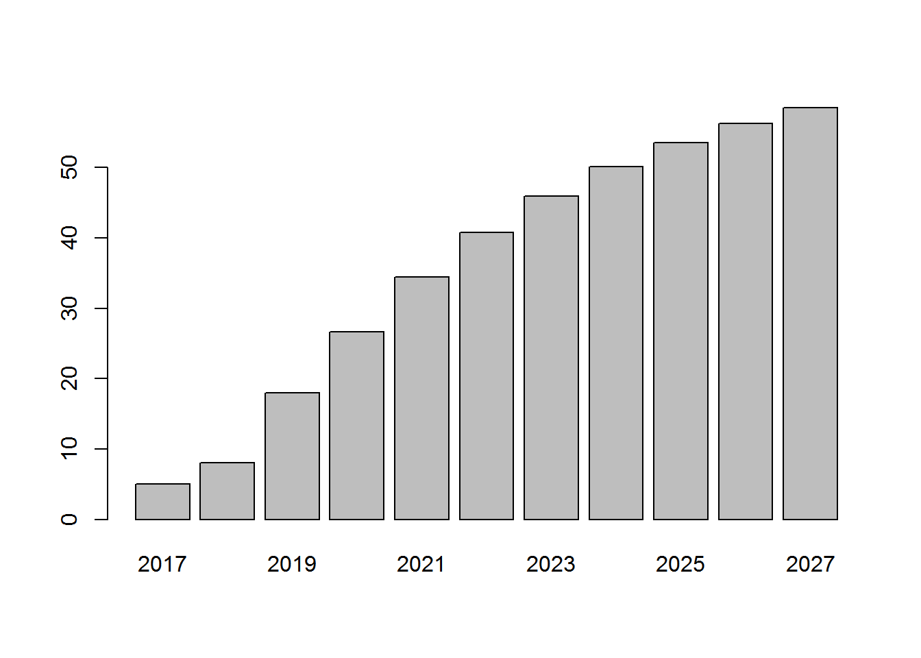 Inactive customers are growing over time.
Plot cold customers over time
barplot(segments[2, ])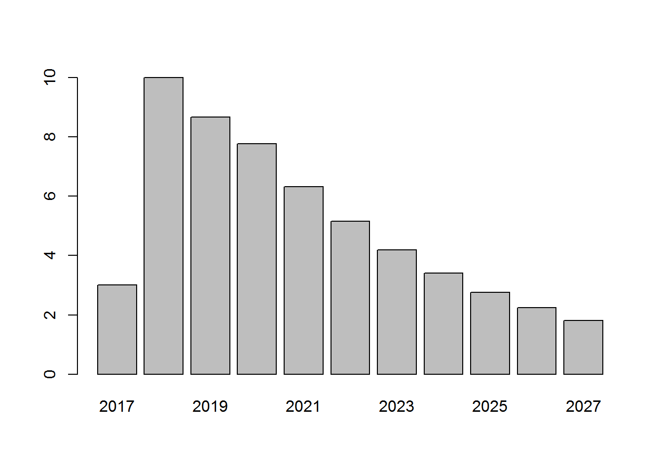 Cold customers grow in 2018, but decline back to 2017 levels by 2027.
The next step in our CLV analysis is to compute the (discounted) Customer Lifetime Value (CLV) of the database. We want to convert the number of customer per segment into monetary value, for each segment. For the Yearly revenue per segment, first create the revenue generated in 2017 for each customer:
revenue_2017 <- df %>% filter(year_of_purchase == 2017) %>%
                group_by(Customer_ID) %>%
                summarize(revenue_2017 = sum(Value))
                # creates a new variable: the sum of purchase amount in 2017

# then merge 2017 customers and 2017 revenue
actual <- merge(df_17, revenue_2017, all.x = TRUE)
actual$revenue_2017[is.na(actual$revenue_2017)] <- 0
Next compute the average revenue per customer for each segment, and store the results in yearly_revenue:
revenue_segment <- aggregate(x = actual$revenue_2017, by = list(df_17$segment), mean)
revenue_segment
Group.1 x1 inactive 0 2 cold 0 3 warm high value 0 4 warm low value 0 5 active high value 516856238 6 active low value 82270716 7 new active 831765604
yearly_revenue <- revenue_segment$x
yearly_revenue
[1] 0 0 0 0 516856238 82270716 831765604
Here we see a new active customer generates $831k of revenue in 2017. Without additional information, we will assume that the revenue per segment remains stable over time. Hence, a new active customer will generate 831k of revenue per year.
Computing the revenue per segment
The next step is to multiply ‘segments’, which contains predictions of segment membership over the next 11 years, by how much revenue each segment generates:
revenue_per_segment <- segments * yearly_revenue    # element-wise multiplication
revenue_per_segment
2017 2018 2019 2020 2021inactive 0 0 0 0 0 cold 0 0 0 0 0 warm high value 0 0 0 0 0 warm low value 0 0 0 0 0 active high value 9820268527 8731485346 7165165424 5868282836 4797885158 active low value 2221309340 2010767076 1621586352 1307730929 1054621717 new active 3327062418 0 0 0 0 2022 2023 2024 2025 2026 inactive 0 0 0 0 0 cold 0 0 0 0 0 warm high value 0 0 0 0 0 warm low value 0 0 0 0 0 active high value 3916825133 3193321152 2600416234 2115406042 1719278923 active low value 850501385 685888213 553135656 446077142 359739631 new active 0 0 0 0 0 2027 inactive 0 cold 0 warm high value 0 warm low value 0 active high value 1396192577 active low value 290112605 new active 0 The active high value customers have generated $9.8 million in 2017.
Computing the total yearly revenue Then we want to know the total yearly revenue (ie. the sum of each column):
yearly_revenue <- colSums(revenue_per_segment)
round(yearly_revenue)
2017 2018 2019 2020 2021 2022 15368640284 10742252423 8786751775 7176013765 5852506875 4767326517 2023 2024 2025 2026 2027 3879209365 3153551890 2561483183 2079018554 1686305182
barplot(yearly_revenue)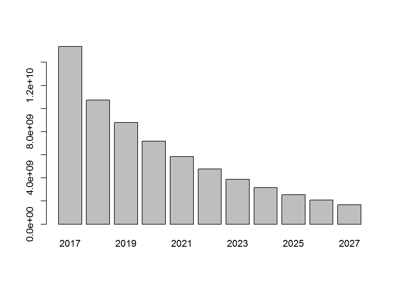
Acme generated 15 billion dollars in 2017. This yearly revenue doesn’t account for any discount rate. Because there will be more and more inactive customers over time (Acme loses customers over time), by the year 2027, the yearly revenue will be only 1.7 million dollars.
Computing the cumulated yearly revenue
cumulated_revenue <- cumsum(yearly_revenue)
round(cumulated_revenue)
2017 2018 2019 2020 2021 2022 15368640284 26110892707 34897644482 42073658248 47926165122 52693491639 2023 2024 2025 2026 2027 56572701005 59726252895 62287736078 64366754632 66053059814
barplot(cumulated_revenue)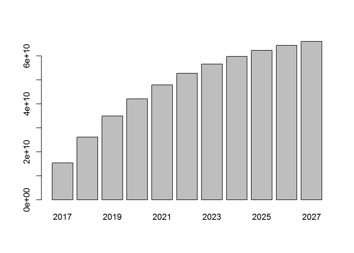
Creating a discount factor A dollar 10 years from now is not worth a dollar today. Let’s create a 10% discount rate vector:
discount_rate <- 0.10
discount <- 1 / ((1 + discount_rate) ^ ((1:11) - 1))
discount
[1] 1.0000000 0.9090909 0.8264463 0.7513148 0.6830135 0.6209213 0.5644739 [8] 0.5131581 0.4665074 0.4240976 0.3855433 Note that the discount rate doesn’t apply to the first year (2017). Then a dollar in 2018 will be worth $0.909 and so on.
Computing the discounted yearly revenue Then we simply multiply the yearly revenue vector by the discount rate vector:
disc_yearly_revenue <- yearly_revenue * discount    # element-wise multiplication
round(disc_yearly_revenue)
2017 2018 2019 2020 2021 2022 15368640284 9765684021 7261778327 5391445353 3997340943 2960134688 2023 2024 2025 2026 2027 2189712556 1618270754 1194950809 881706817 650143647
The yearly revenue in 2027 becomes 650 million USD. That’s how much money in today’s worth is going to be generated in 2027, for two reasons:
It is a revenue in 10 years, so it needs to be discounted It’s in 10 years, meaning many customers will have left and won’t be active anymore
barplot(disc_yearly_revenue)
lines(yearly_revenue)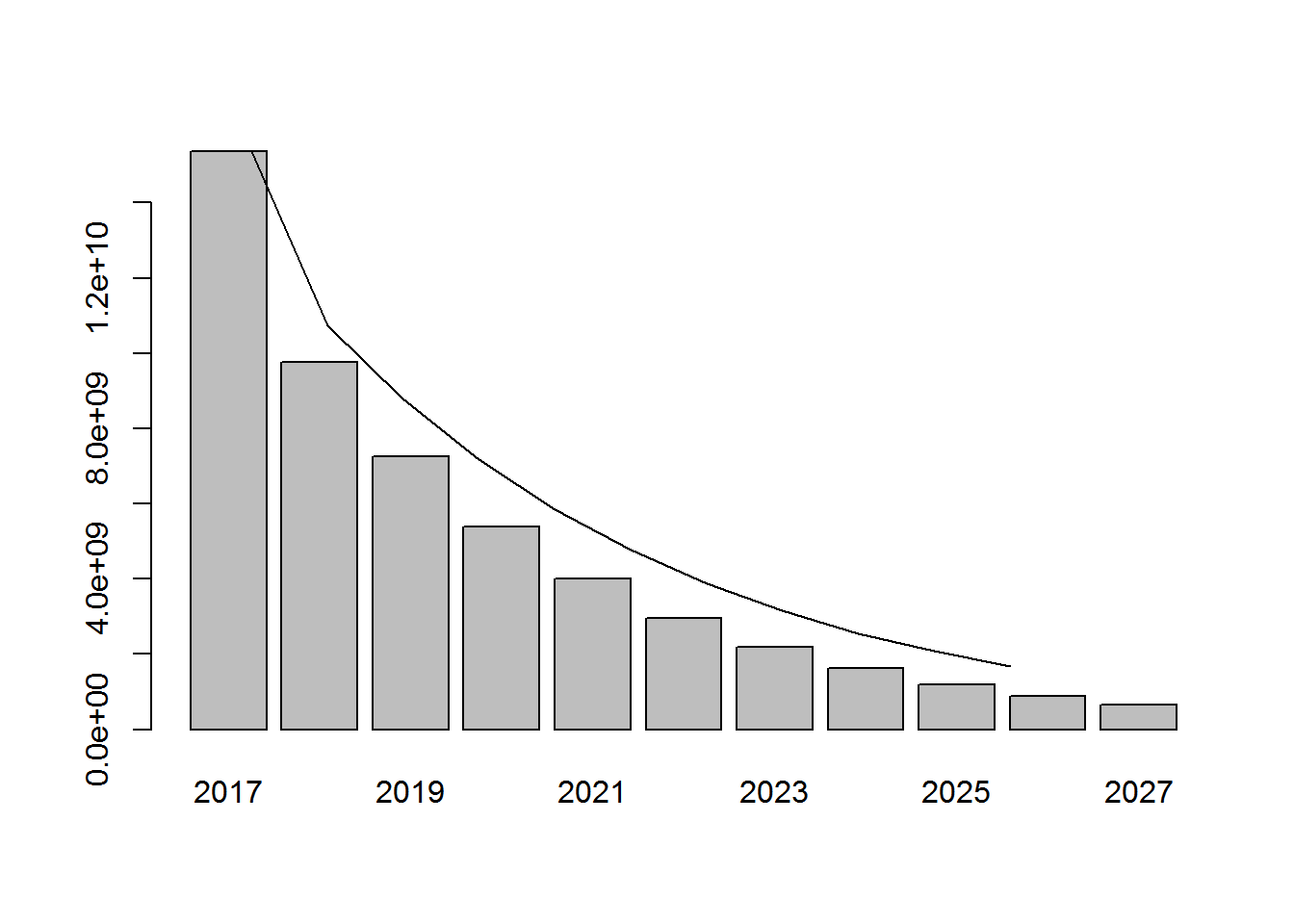
The barchart represents the discounted yearly revenues whereas the line represents the undiscounted yearly revenues. The further away in the future you get the revenue, the less worth it is in today’s dollar.
Computing discounted cumulated yearly revenue
disc_cumulated_revenue <- cumsum(disc_yearly_revenue)
round(disc_cumulated_revenue)
2017 2018 2019 2020 2021 2022 15368640284 25134324305 32396102631 37787547985 41784888928 44745023616 2023 2024 2025 2026 2027 46934736172 48553006926 49747957735 50629664553 51279808199
barplot(disc_cumulated_revenue)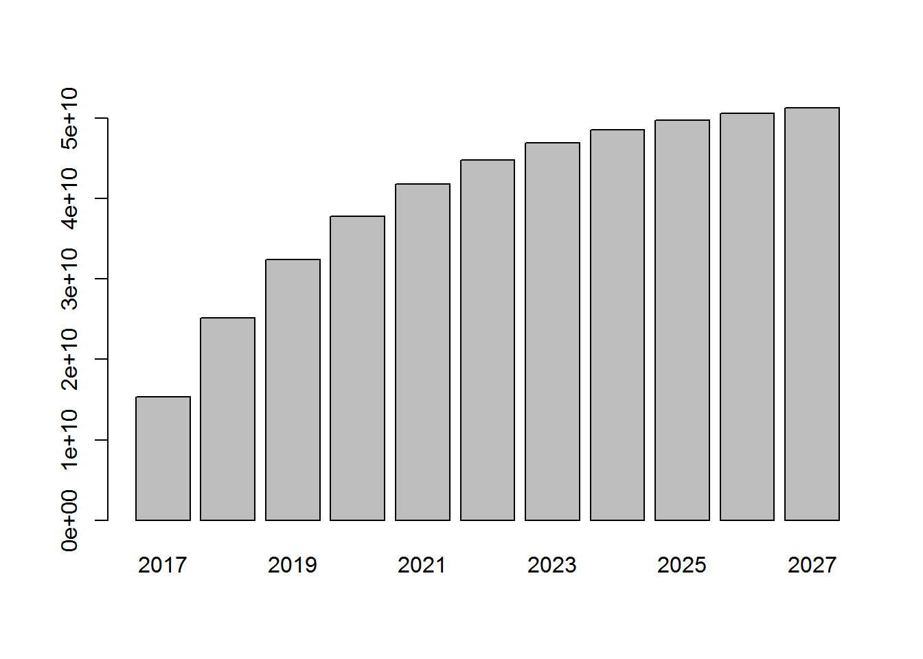
How much is the customer database worth? Over the next 10 years, how much is the customer database worth? What is the true value, the discounted cumulated value of my database in terms of expected revenue of the next 10 years?
disc_cumulated_revenue[11] - yearly_revenue[1] 2027 35911167915
It is the discounted cumulated yearly revenue in 10 years (in 2027) minus the yearly revenue from today (2017), which already happened. The answer is 35 billion dollars. This is the value of the database in today’s dollars in terms of how much revenue it will generate over the next 10 years.