Chapter 9 Finance
9.1 Financial Calculations
9.1.1 Amortization Period
Amortizatiion Period (amort.period) solves for either the number of payments, the payment amount, or the amount of a loan. The payment amount, interest paid, principal paid, and balance of the loan are given for a specified period.
Usage
amort.period(Loan=NA,n=NA,pmt=NA,i,ic=1,pf=1,t=1)
Arguments
Loan = loan amount
n = the number of payments/periods
pmt = value of level payments
i = nominal interest rate convertible ic times per year
ic = interest conversion frequency per year
pf = the payment frequency- number of payments per year
t = the specified period for which the payment amount, interest paid, principal paid, and loan balance are solved for
Value
Returns a matrix of input variables, calculated unknown variables, and amortization figures for the given period.
Note
Assumes that payments are made at the end of each period.
One of n, pmt, or Loan must be NA (unknown).
If pmt is less than the amount of interest accumulated in the first period, then the function will stop because the loan will never be paid off due to the payments being too small.
If the pmt is greater than the loan amount plus interest accumulated in the first period, then the function will stop because one payment will pay off the loan.
t cannot be greater than n.
Acme need to invest in equipment to increase its production of Triple-Strength Battleship Steel Armor Plates and would like to explore financing options to fund the expansion. Let’s use amort.period to calculate different aspects of the potential loan.
Assuming the loan amount of 1,000,000, for a period of 5 years, and an interest rate of 2%, what is the interest, what is the interest paid, principal paid and balance at year 3?
library(FinancialMath)

amort.period(Loan=1000000,n=5,i=.02,t=3) AmortizationLoan 1000000.00 PMT 212158.39 Eff Rate 0.02 Years 5.00 At Time 3: 3.00 Int Paid 12236.80 Princ Paid 199921.59 Balance 411918.45
Assuming a payment of 100,000, for a period of 5 years, and an interest rate of 2%, making 12 payments per year, what is the interest paid, principal paid and balance at year 3?
amort.period(n=5,pmt=30,i=.02,t=3,pf=12) AmortizationLoan 149.259643 PMT 30.000000 Eff Rate 0.020000 i^(12) 0.019819 Periods 5.000000 Years 0.416667 At Time 3: 3.000000 Int Paid 0.148153 Princ Paid 29.851847 Balance 59.851684
Assuming a payment of 1,000,000, a payment of 100,000 and an interest conversion of 1, an interest rate of 2 %, what is the interest paid, principal paid and balance at year 3?
amort.period(Loan=1000000,pmt=100000,ic=1,i=.02,t=3) AmortizationLoan 1.000000e+06 PMT 1.000000e+05 Eff Rate 2.000000e-02 Years 1.126838e+01 At Time 3: 3.000000e+00 Int Paid 1.676800e+04 Princ Paid 8.323200e+04 Balance 7.551680e+05
9.1.2 Amortization Table
Amortizatiion Table (amort.table) produces an amortization table for paying off a loan while also solving for either the number of payments, loan amount, or the payment amount. In the amortization table the payment amount, interest paid, principal paid, and balance of the loan are given for each period. If n ends up not being a whole number, outputs for the balloon payment, drop payment and last regular payment are provided. The total interest paid, and total amount paid is also given. It can also plot the percentage of each payment toward interest vs. period.
Usage
amort.table(Loan=NA,n=NA,pmt=NA,i,ic=1,pf=1,plot=FALSE)
Arguments
Loan = loan amount
n = the number of payments/periods
pmt = value of level payments
i = nominal interest rate convertible ic times per year
ic = interest conversion frequency per year
pf = the payment frequency- number of payments per year
plot = tells whether or not to plot the percentage of each payment toward interest vs. period
The output is a a list of two components.
Schedule: A data frame of the amortization schedule.
Other: A matrix of the input variables and other calculated variables.
Note
Assumes that payments are made at the end of each period.
One of n, Loan, or pmt must be NA (unknown).
If pmt is less than the amount of interest accumulated in the first period, then the function will stop because the loan will never be paid off due to the payments being too small.
If pmt is greater than the loan amount plus interest accumulated in the first period, then the function will stop because one payment will pay off the loan.
Examples
library(FinancialMath)
amort.table(Loan=1000,n=2,i=.005,ic=1,pf=1)
$Schedule Payment Interest Paid Principal Paid Balance 1 503.75 5.00 498.75 501.25 2 503.75 2.51 501.25 0.00
$Other Details Loan 1000.000 Total Paid 1007.510 Total Interest 7.510 Eff Rate 0.005
amort.table(Loan=100,pmt=40,i=.02,ic=2,pf=2,plot=FALSE)$Schedule Year Payment Interest Paid Principal Paid Balance 1 0.50 40.00 1.00 39.00 61.00 2 1.00 40.00 0.61 39.39 21.61 2.54 1.27 21.73 0.12 21.61 0.00
$Other Details Loan 100.00000 Total Paid 101.73000 Total Interest 1.73000 Balloon PMT 61.61000 Drop PMT 21.82610 Last Regular PMT 21.72738 Eff Rate 0.02010 i^(2) 0.02000
amort.table(Loan=NA,pmt=102.77,n=10,i=.005,plot=TRUE)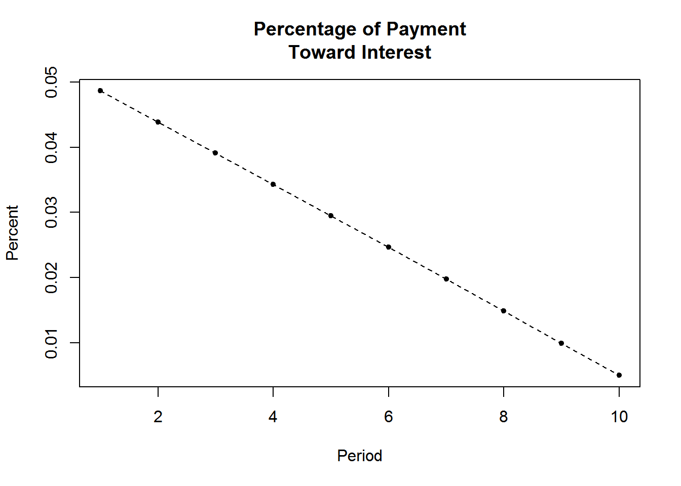 $Schedule Payment Interest Paid Principal Paid Balance 1 102.77 5.00 97.77 902.22 2 102.77 4.51 98.26 803.97 3 102.77 4.02 98.75 705.22 4 102.77 3.53 99.24 605.97 5 102.77 3.03 99.74 506.23 6 102.77 2.53 100.24 405.99 7 102.77 2.03 100.74 305.25 8 102.77 1.53 101.24 204.01 9 102.77 1.02 101.75 102.26 10 102.77 0.51 102.26 0.00
$Other Details Loan 999.9944 Total Paid 1027.7000 Total Interest 27.7100 Eff Rate 0.0050
9.1.3 IRR Internal Rate of Return
IRR calculates internal rate of return for a series of cash flows, and provides a time diagram of the cash flows.
Usage
IRR(cf0,cf,times,plot=FALSE)
Arguments
cf0 = cash flow at period 0
cf = vector of cash flows
times = vector of the times for each cash flow
plot = option whether or not to provide the time diagram
Note
Periods in t must be positive integers.
Uses polyroot function to solve equation given by series of cash flows, meaning that in the case of having a negative IRR, multiple answers may be returned.
Examples
library(FinancialMath)
IRR(cf0=1,cf=c(1,2,1),times=c(1,3,4))
[1] 0.7943097
IRR(cf0=100,cf=c(1,1,30,40,50,1),times=c(1,1,3,4,5,6))[1] 0.05166628
9.1.4 NPV Net Present Value
Net Present Value (NPV) calculates the net present value for a series of cash flows, and provides a time diagram of the cash flows.
Usage
NPV(cf0,cf,times,i,plot=FALSE)
Arguments
cf0 = cash flow at period 0
cf = vector of cash flows
times = vector of the times for each cash flow
i = interest rate per period
plot = tells whether or not to plot the time diagram of the cash flows
Note
The periods in t must be positive integers.
The lengths of cf and t must be equal.
Examples
library(FinancialMath)
NPV(cf0=100,cf=c(50,40),times=c(3,5),i=.01)
[1] -13.41187
NPV(cf0=100,cf=50,times=3,i=.05)[1] -56.80812
NPV(cf0=100,cf=c(50,60,10,20),times=c(1,5,9,9),i=.045)[1] 16.18109
9.1.5 TVM Time Value of Money
Time Value of Money (TVM) solves for the present value, future value, time, or the interest rate for the accumulation of money earning compound interest. It can also plot the time value for each period.
Usage
TVM(pv=NA,fv=NA,n=NA,i=NA,ic=1,plot=FALSE)
Arguments
pv = present value
fv = future value
n = number of periods
i = nominal interest rate convertible ic times per period
ic = interest conversion frequency per period
plot = tells whether or not to produce a plot of the time value at each period
Returning a matrix of the input variables and calculated unknown variables.
Note that exactly one of pv, fv, n, or i must be NA (unknown).
Examples
library(FinancialMath)
TVM(pv=10,fv=20,i=.05,ic=2,plot=TRUE)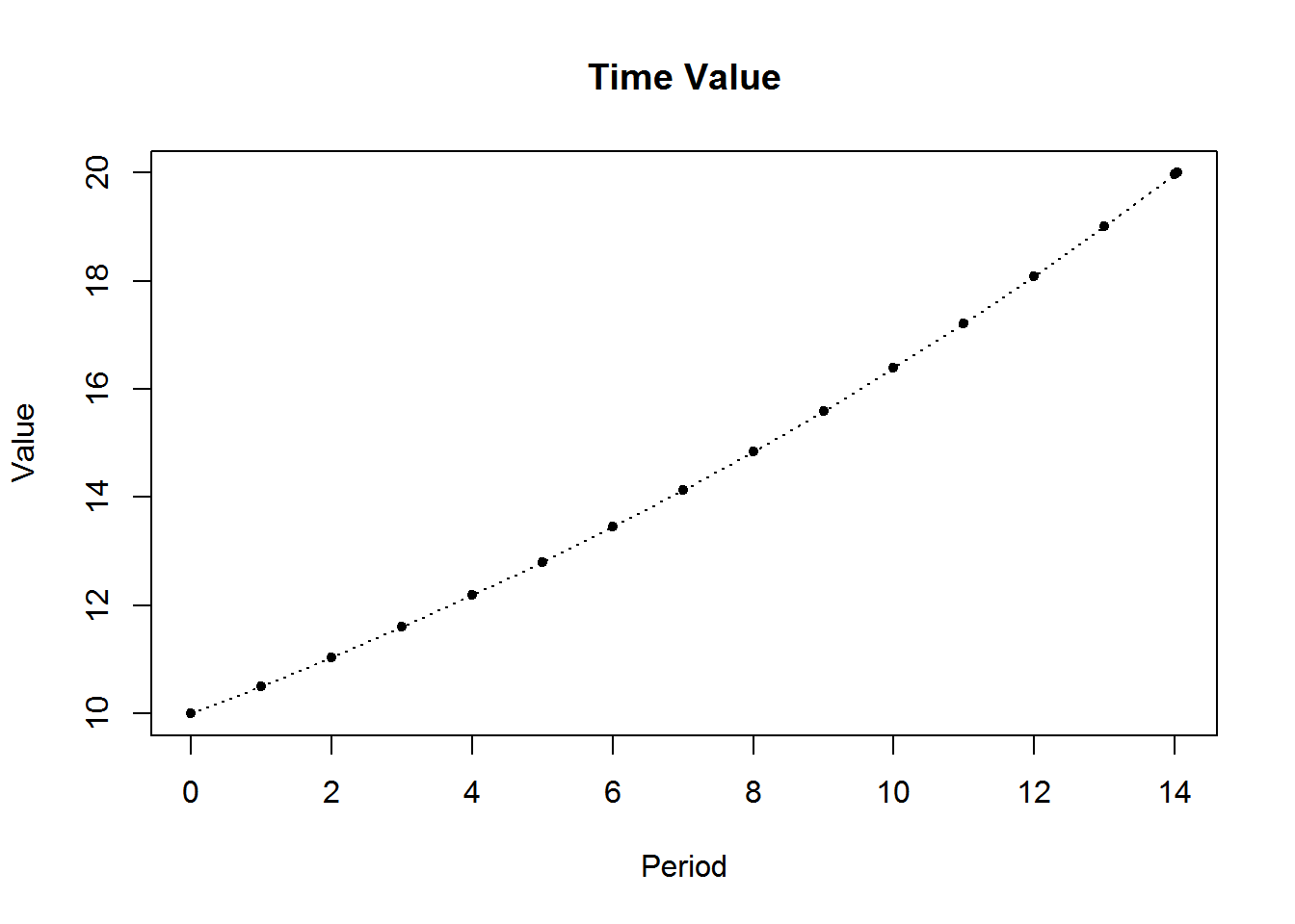 TVM PV 10.000000 FV 20.000000 Periods 14.035517 Eff Rate 0.050625 i^(2) 0.050000
TVM(pv=50,n=5,i=.04,plot=TRUE)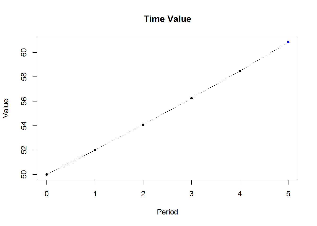 TVM PV 50.00000 FV 60.83265 Periods 5.00000 Eff Rate 0.04000
9.2 Time Series Basics
R has a broad capabilities for analyzing time series data. Here we describe the creation of a time series, seasonal decomposition, modeling with exponential and ARIMA models, and forecasting with the forecast package.
The first step is to creating a time series. The ts() function will convert a numeric vector into an R time series object. The format is ts(vector, start=, end=, frequency=) where start and end are the times of the first and last observation and frequency is the number of observations per unit time (1=annual, 4=quartly, 12=monthly, etc.).
As part of the planning process, Acme would like to develop a 5 year forecast of its sales volume. Perhaps no type of forecasting is more prevalent in planning that Time Series forecasting, so we’ll start there. Let’s return to the sales_hist data set, reviewed previously.
df <- read.csv('https://raw.githubusercontent.com/jmonroe252/RforBusiness/master/sales_hist.csv', stringsAsFactors = FALSE)

#### Select and format the Units Field
library(dplyr)
## Warning: package 'dplyr' was built under R version 3.4.2##
## Attaching package: 'dplyr'## The following objects are masked from 'package:stats':
##
## filter, lag## The following objects are masked from 'package:base':
##
## intersect, setdiff, setequal, uniondf %>%
select(Units) %>%
mutate(Units = as.numeric(Units)) -> dfCreate a time series object from Jan 2002 to Dec 2017:
ts <- ts(df, start=c(2002, 1), end=c(2017, 12), frequency=12) Subset the time series (January 2014 to December 2017):
ts2 <- window(ts, start=c(2014, 1), end=c(2017, 12)) Plot the time series
plot(ts2)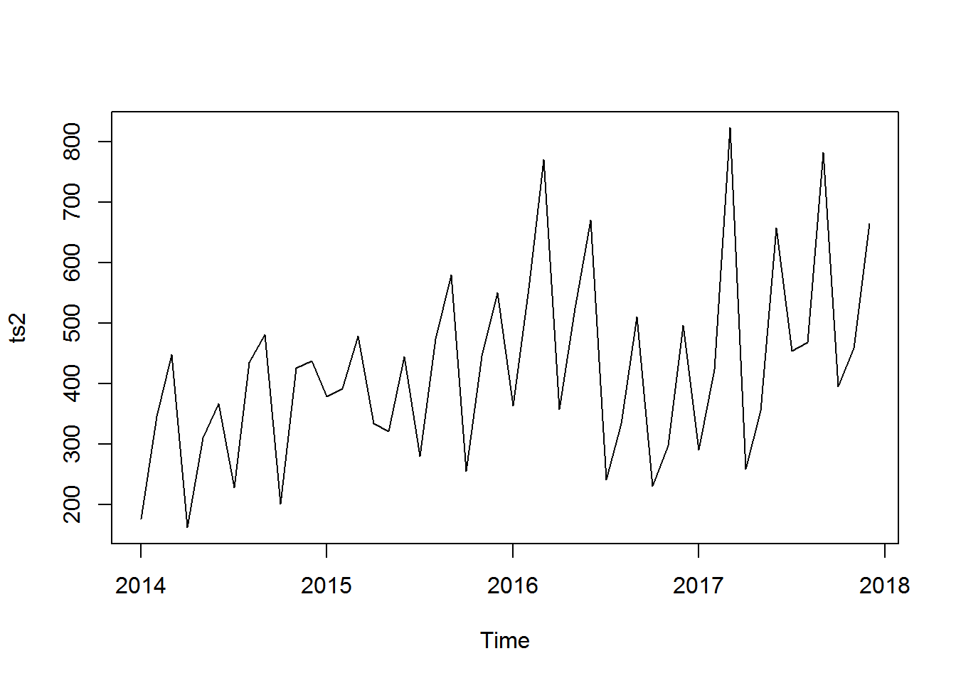
Seasonal Decomposition is a time series with additive trend, seasonal, and irregular components and can be decomposed using the stl() function. Note that a series with multiplicative effects can often by transformed into series with additive effects through a log transformation (i.e., newts <- log(ts)).
An example of Seasonal decomposition is:
fit <- stl(ts, s.window="period")
plot(fit)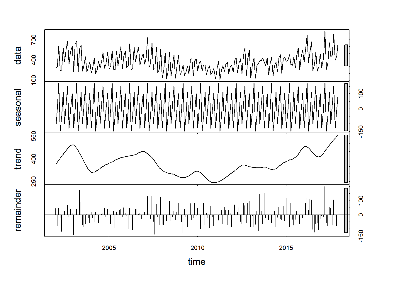
Create a Month Plot
monthplot(ts)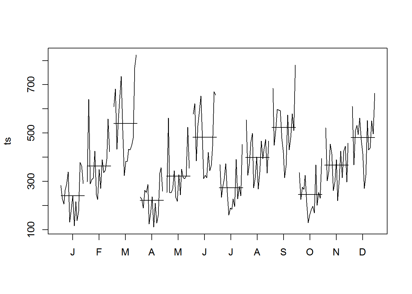
And a seasonal plot, included in the forecast package.
library(forecast)
seasonplot(ts)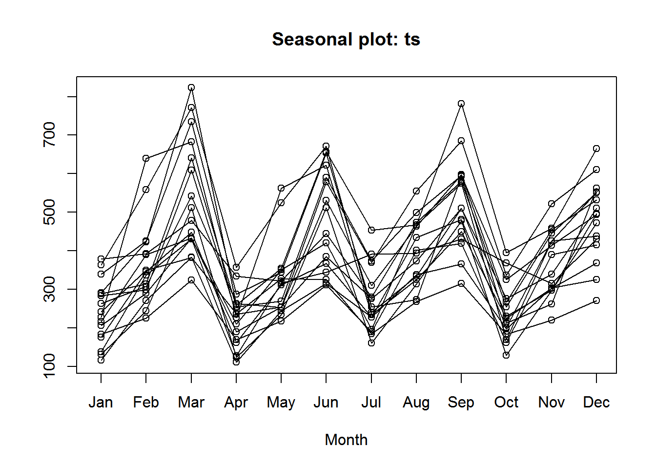
Let’s now develop a forecast of Acme’s unit volume. For this, we’ll return to the forecast package. Both the HoltWinters() function in the base installation, and the ets() function in the forecast package, can be used to fit exponential models.
library(forecast)
#### simple exponential - models level
fit <- HoltWinters(ts, beta=FALSE, gamma=FALSE)
#### double exponential - models level and trend
fit <- HoltWinters(ts, gamma=FALSE)
#### triple exponential - models level, trend, and seasonal components
fit <- HoltWinters(ts)

#### predictive accuracy
accuracy(fit)

#### predict next three future values
library(forecast)
forecast(fit, 5)
plot(forecast(fit, 5))
The arima() function can be used to fit an autoregressive integrated moving averages model (ARIMA).
Other useful functions include:
lag(ts, k) lagged version of time series, shifted back k observations
diff(ts, differences=d) difference the time series d times
ndiffs(ts) Number of differences required to achieve stationarity (from the forecast package)
acf(ts) autocorrelation function
pacf(ts) partial autocorrelation function
adf.test(ts) Augemented Dickey-Fuller test. Rejecting the null hypothesis suggests that a time series is stationary (from the tseries package)
Box.test(x, type=“Ljung-Box”) Pormanteau test that observations in vector or time series x are independent
Note that the forecast package has somewhat nicer versions of acf() and pacf() called Acf() and Pacf() respectively.
#### fit an ARIMA model of order P, D, Q
fit <- Arima(ts, order=c(1, 0, 0))

#### predictive accuracy
library(forecast)
accuracy(fit)
ME RMSE MAE MPE MAPE MASETraining set -0.008716872 148.1198 120.3377 -18.84267 40.01171 1.261548 ACF1 Training set -0.00126353
#### predict next 5 observations
forecast(fit, 5)
Point Forecast Lo 80 Hi 80 Lo 95 Hi 95Jan 2018 365.9594 175.1398 556.7790 74.12607 657.7928 Feb 2018 371.6650 180.8107 562.5193 79.77851 663.5514 Mar 2018 371.5561 180.7018 562.4104 79.66963 663.4426 Apr 2018 371.5582 180.7039 562.4125 79.67171 663.4447 May 2018 371.5581 180.7038 562.4125 79.67167 663.4446
plot(forecast(fit, 5))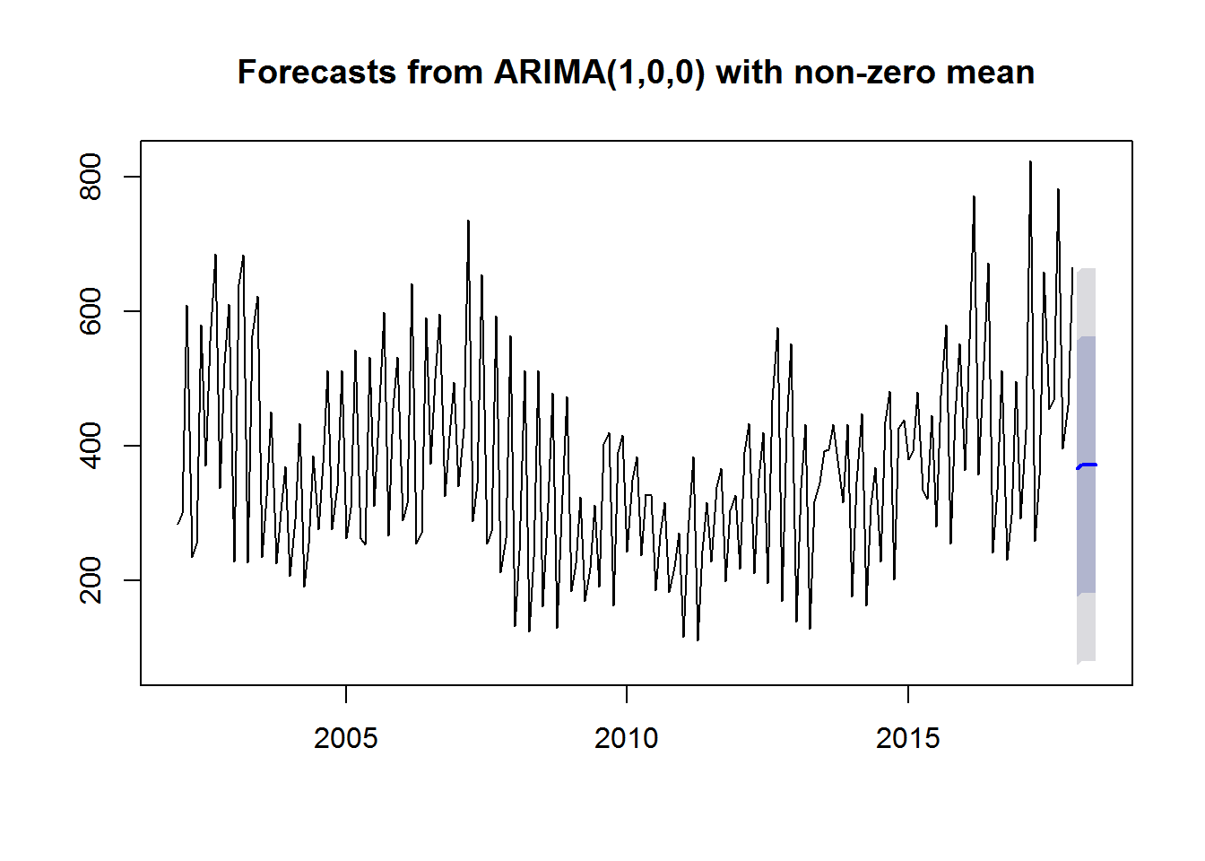
The forecast package provides functions for the automatic selection of exponential and ARIMA models. The ets() function supports both additive and multiplicative models. The auto.arima() function can handle both seasonal and nonseasonal ARIMA models. Models are chosen to maximize one of several fit criteria.
#### Automated forecasting using an exponential model
fit <- ets(ts)

#### Automated forecasting using an ARIMA model
fit <- auto.arima(ts)