Chapter 9 Selection bias
9.0.1 R packages required for this chapter
library(knitr)
library(tidyverse)
library(dagitty)
library(ggdag)
library(patchwork)
9.1 Introduction
Selection bias is introduced by the improper (non random) selection of individuals, such that the sample of cases and controls are not drawn from the same reference population. If the selection of cases and controls is not done independently of the exposure, then when you compare exposure distributions any observed differences are a combination of a true effect and an artifact of the way the data was collected (i.e., differential selection into the study sample). In other words, selection bias can lead to potential spurious statistical analyses of exposure / outcome associations by the method of samples selection thereby negatively affecting internal validity. Selection bias can also have a negative impact on external validity.
The following [cartoon]((https://youtu.be/p52Nep7CBdQ) may help convincingly illustrate the concept.
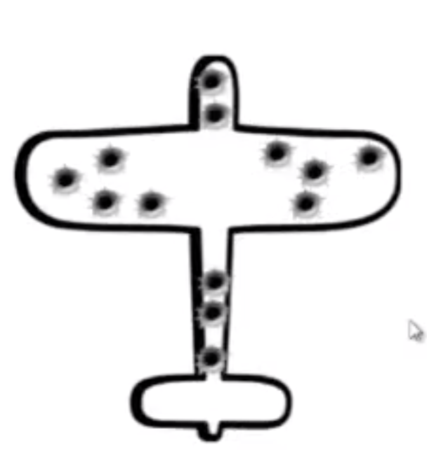
Figure 2.1: Summary of damaged airplanes
This cartoon represented the damage of returning bombers after raids during WWII. The statistician, Abraham Wald, was asked to help the British decide where to add armor to their bombers.
Is it obvious where the armour should be placed?
After analyzing the records, he recommended adding armor to the places where there was no damage!
This may seem odd at first, but Wald realized his data for analysis came from bombers that survived. Those that were shot down over enemy territory were not part of their sample and the undamaged areas on the survivors showed where the lost planes must have been hit because the planes hit in those areas did not return from their missions. This is known as survivorship bias, a form of selection bias. The full account of Wald’s work on this problem can be found here.
9.2 Selction bias in case control designs
Selection bias occurs when exposure and disease outcome both affect participation in the study. It is most easily appreciated in case control designs and arises when cases and controls are not selected independently of exposure. Graphically this shown by examining the relationship between the 2X2 tables of the reference (target) and the study (sample) population. If any of the cells of the study population are not filled in direct proportion to the target population, selection bias may occur.
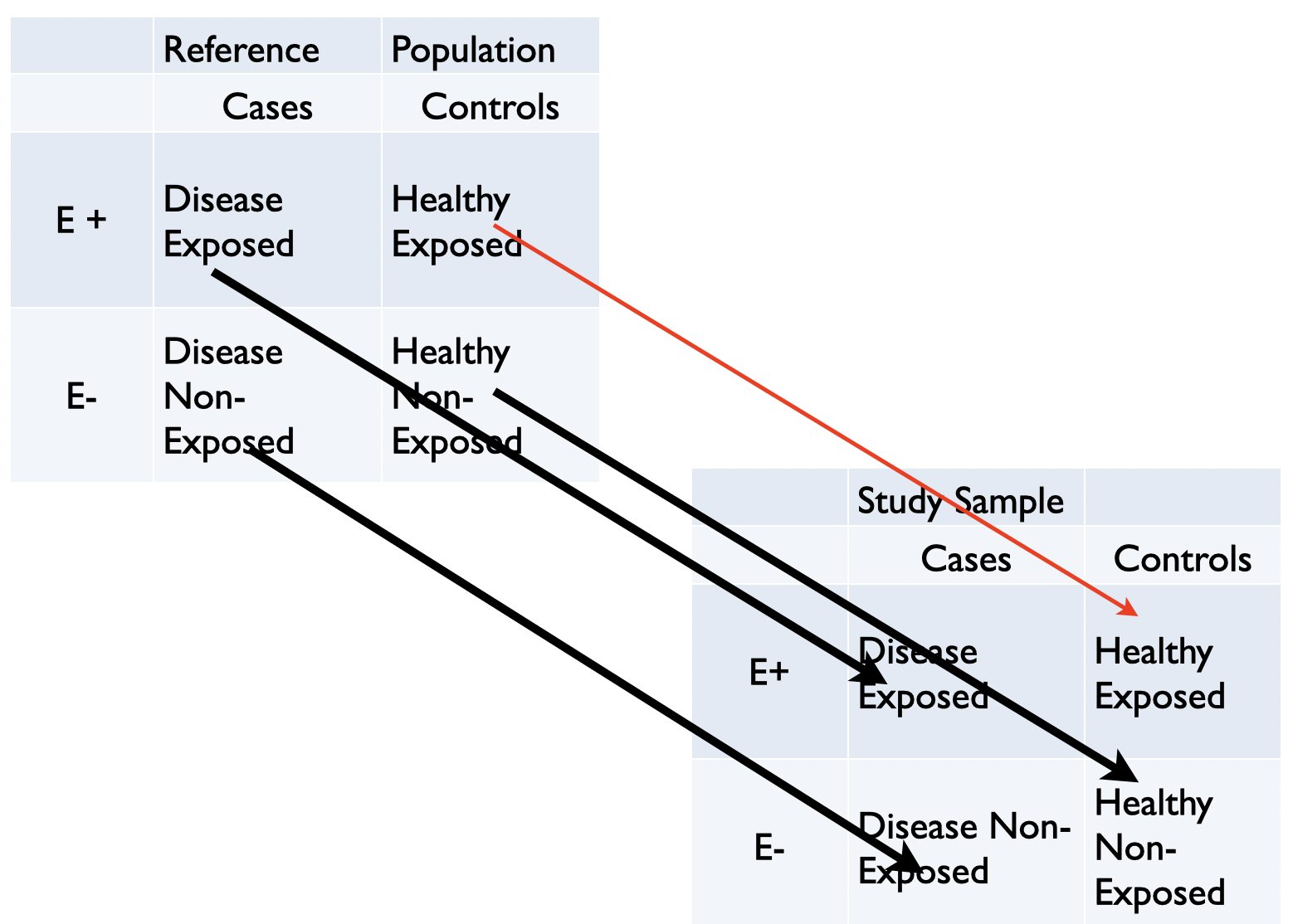
Figure 3.4: Graphical display of selection bias in case control design
Selection bias can arise from other research designs, including RCTs but may occasionally be difficult to identify and are frequently overshadowed by other bias. Selection bias is nevertheless ubiquitous and has the potential to lead research astray. Part of the difficulty appreciating selection bias is that historically this bias has been identified by specific examples rather than by a general formulation.
Classic examples include healthy-worker bias, volunteer bias, differential loss-to-followup, depletion of susceptibles, incidence - prevalence bias, nonresponse bias and Berkson bias, a particular form of selection bias when using hospital controls.
Newer examples examples include index event bias, also known as collider stratification bias (see Chapter 7.3) and immortal time bias which has both a misclassification & selection component and is especially problematic in especially in pharmacoepidemiologic studies.
There are a number of excellent recent review articles on selection bias(Smith 2020)(Haneuse 2016)(Hernan, Hernandez-Diaz, and Robins 2004).
9.3 Comparison of confounding, mediation and selection bias with DAGs
Confounding and selection bias are two important biases, and since their occurrence may occasionally be less than obvious, DAGs provide an explicit means to distinguish between them. Confounding is the result of a common cause while selection bias is the result of conditioning on a common effect. Confounding can then be appreciated as a state of nature while selection bias is an artifact of the research process but both result in the noncomparability (also referred to as lack of exchangeability) between the exposed and the unexposed.
The following DAGs shows the relationships underlying confounding, mediation and selection bias.
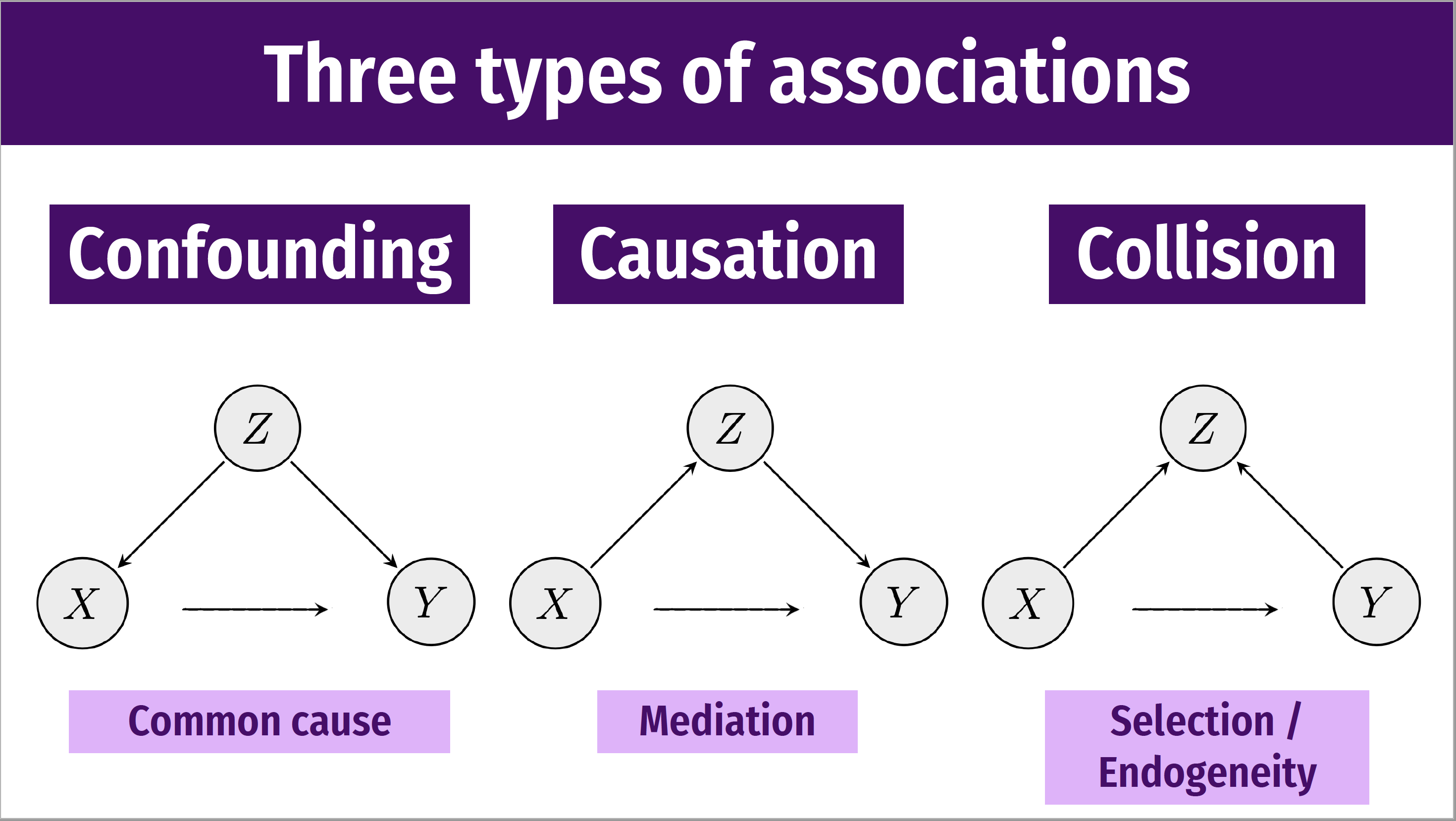
Figure 3.5: Types of associations
Following Chapter 7.3, we can also use the daggity package to draw these DAGs.
# example 1
dag <- dagitty("dag {
  X -> Y
  Z -> X
  Z ->  Y
               }")

coordinates( dag ) <-  list(
  x=c(X=1, Z=3, Y=5),
  y=c(X=1, Z=3, Y=1) )

dag <- tidy_dagitty(dag)
ex1 <- ggdag(dag, layout = "circle") + theme_dag_blank(plot.caption = element_text(hjust = 1)) + geom_dag_node(color="pink") + geom_dag_text(color="white") +
  ggtitle("a) Confounding ") +
  labs(caption = "Common cause")

# example 2
dag <- dagitty("dag {
  X -> Y
  X -> Z
  Z ->  Y
               }")

coordinates( dag ) <-  list(
  x=c(X=1, Z=3, Y=5),
  y=c(X=-.5, Z=1, Y=-.5) )

ex2 <- ggdag(dag, layout = "circle") + theme_dag_blank(plot.caption = element_text(hjust = 1)) + geom_dag_node(color="pink") + geom_dag_text(color="white") +
  ggtitle("b) Causation") +
  labs(caption = "Mediation")

# example 3
dag <- dagitty("dag {
  X -> Y
  X -> Z
  Y ->  Z
               }")

coordinates( dag ) <-  list(
  x=c(X=1, Z=3, Y=5),
  y=c(X=-.5, Z=1, Y=-.5) )

ex3 <- ggdag(dag, layout = "circle") + theme_dag_blank(plot.caption = element_text(hjust = 1)) + geom_dag_node(color="pink") + geom_dag_text(color="white") +
  ggtitle("c) Collision") +
  labs(caption = "Selection /\nEndogeneity")

ex1 + ex2 + ex3 +
  plot_annotation(title = 'Causal diagrams - confounder, mediator and selection bias')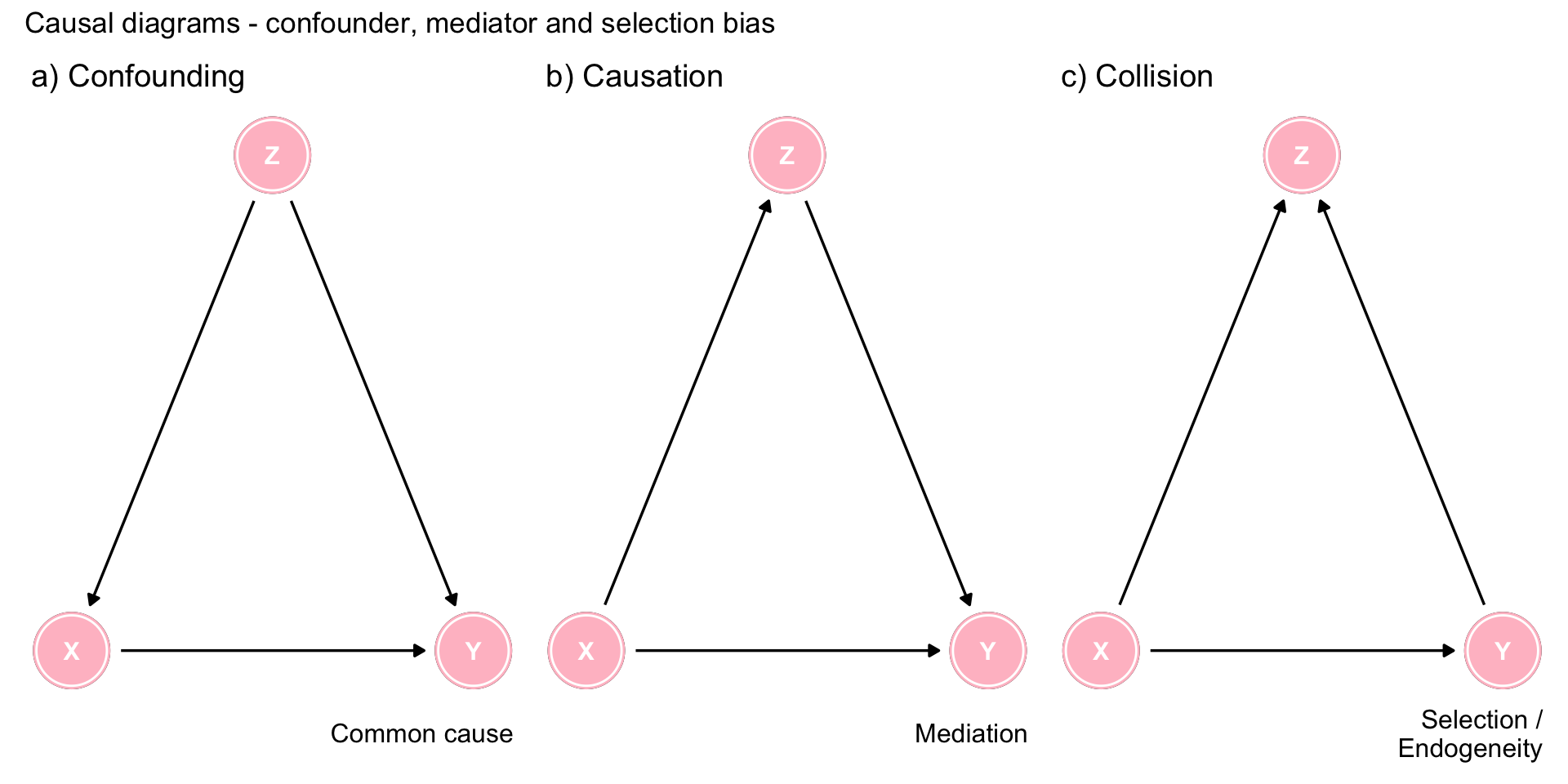
Figure 9.1: Three types of associations
9.4 Case control example - Berkson bias
Consider a case-control study of the association between postmenopausal estrogens and myocardial infarction (MI) where controls are chosen from a hospitalized population. This population may not be representative of the overall taeget population. For example, hospital controls may have over sample of hip fractures. Estrogens are known to be protective the incidence of hip fractures, so controls are less likely to be on estrogens than a MI case, even if estrogen exposure does not cause MI.
DAGs to represent this scenario are asfollows
coords <-  list(
  x=c(E=1, F=2, D=2, S=3),
  y=c(E=1, F=1.2, D=1, S=1) )

dag <- dagify(F ~ E, S ~ F + D, coords = coords)
dag1 <- dag %>% ggdag_drelationship("E", "D") + theme_bw() + ggtitle("a) D and E are d-spearated (in nature)")
dag2 <- dag %>% ggdag_drelationship("E", "D", controlling_for = "S") + theme_bw() + ggtitle("b) D and E are d-connected \n(conditional on S)") +
  labs(caption = "E = estrogen \nD = MI \nF = hip fracture \nS = selected for study")

dag1 + dag2 +
plot_annotation(title = 'DAGs showing Berkson bias') 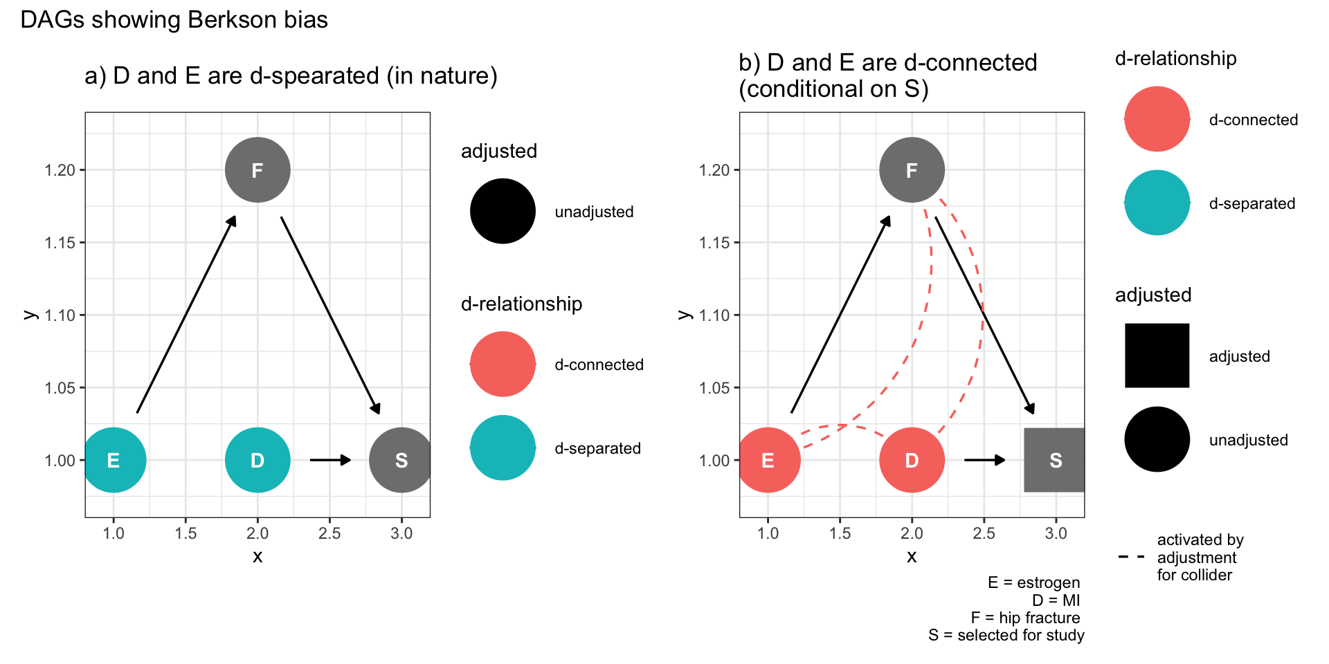
Figure 9.2: Selection bias (Berkson bias)
Figure 9.2a shows no relationship between the exposure (E) and the outcome (D) but once there is conditioning on being selected into the study, a spurious association is created due to collidor stratification. In fact, the ggdag package automatically shows the spurious assocations (dotted lines in Figure 9.2b)
Q: Can a properly randomized clinical trial (RCT) also suffer from selection bias?
A: Yes. Selective lost to follow-up can lead to selection bias. As it is a RCT there are no confounders between E and D. However imagine that exposure to one of the interventions leads to increased side effects (F) which in turn leads to patients dropping out of the study, the equivalent of conditioning on S. In fact this scenario is captured by the
same DAG as Figure 9.2b, demonstrating opening of a spurious backdoor association.
Notice that within this model S could also represent other causes for missingness explaining other biases such as non-response, volunteer, self selection, or healthy worker.
This also explains why complete cases as a means of dealing with missing data is likely to give biased results.
Remember, RCTs can suffer from the same selection biases as observational studies
9.5 Other forms of selection bias as defined by DAGs
In each case, the left hand Figure repesents the causal structure and assuje exposure (D) and outcome (D) are d-separated. While the right sided Figure shows conditioning on study selection leads E and D to become d-connected.
9.5.1 Survival bias
Consider a study of dementia (D) where the exposure to be investigated is physical activity (E) and there exist measured or unmeasured variables (F) associated with both survival (S) and dementia. If physical activity leads to improved survival (S) then a study of older individuals, in other words conditioning on survival, may induce a spurious association between dementia and physical activity. This may result in an association when none truly exists or may modify, to the point of actual reversal, a true association.
coords <-  list(
  x=c(E=1, F=2.5, D=3, S=2),
  y=c(E=1, F=1.2, D=1, S=1) )

dag <- dagify(D ~ F, S ~ F + E, coords = coords)
dag1 <- dag %>% ggdag_drelationship("E", "D") + theme_bw() + ggtitle("a) D and E are d-spearated (in nature)")
dag2 <- dag %>% ggdag_drelationship("E", "D", controlling_for = "S") + theme_bw() + ggtitle("b) D and E are d-connected \n(conditional on S)") +
  labs(caption = "E = physical activity \nD = dementia \nF = other variables e.g. smoking status \nS = selected for study based on survival")

dag1 + dag2 +
plot_annotation(title = 'DAGs showing survival bias') 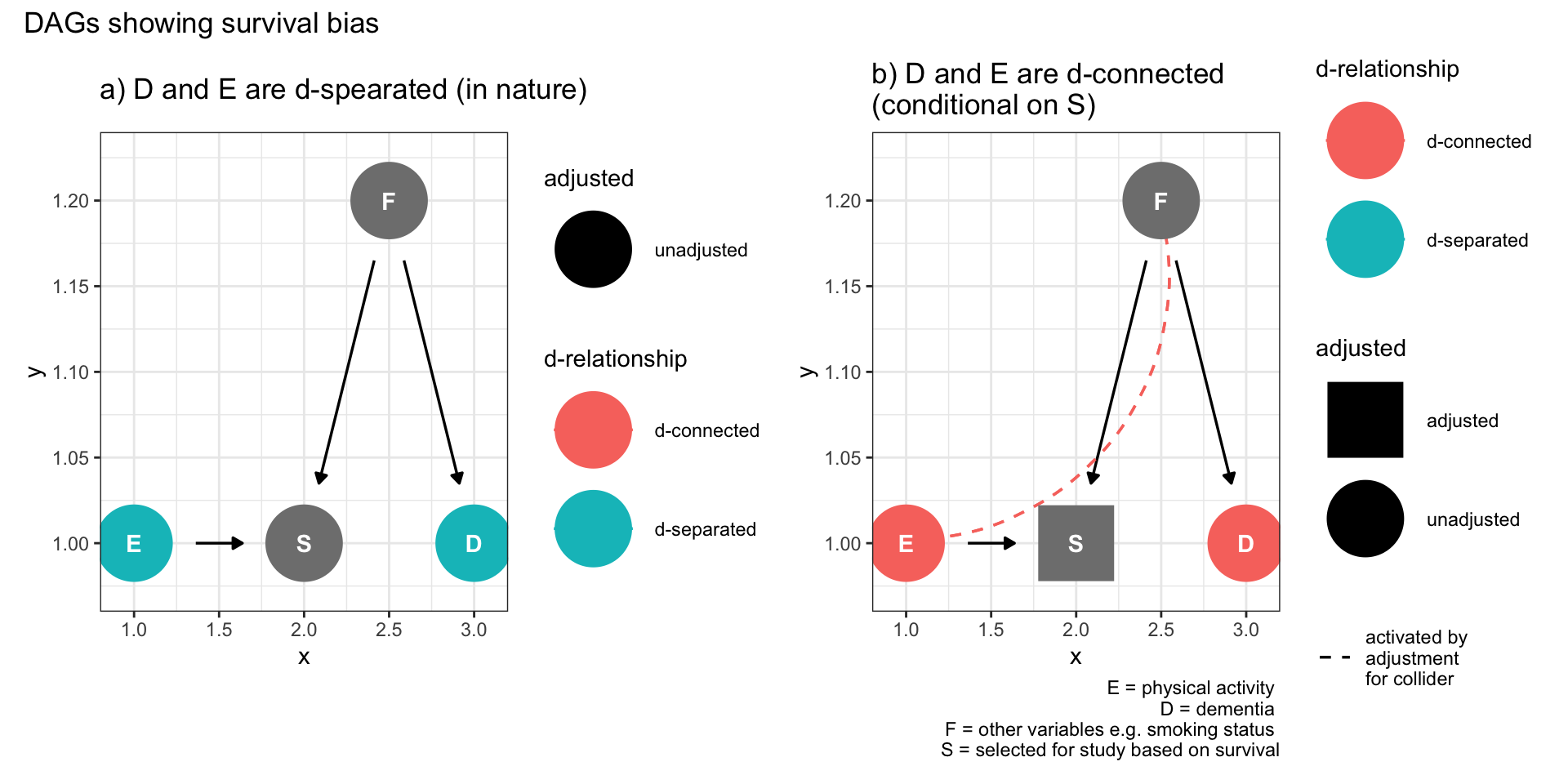
Figure 9.3: Selection bias (survival bias)
9.5.2 Prevalent user bias
Here E is initiation of a drug, E1 is continued use, and S is selection into a study of prevalent users. F is a set of common causes of continued use and the outcome Y, such as underlying health conditions, could lead to selection bias if not taken into account.
coords <-  list(
  x=c(E=1, F=2.5, S=3, E1=2, D=4),
  y=c(E=1, F=1.2, S=1, E1=1, D=1) )

dag <- dagify(E1 ~ E + F, S ~ E1, D ~ F, coords = coords)
dag1 <- dag %>% ggdag_drelationship("E", "D") + theme_bw() + ggtitle("a) D and E are d-spearated (in nature)")
dag2 <- dag %>% ggdag_drelationship("E", "D", controlling_for = "S") + theme_bw() + ggtitle("b) D and E are d-connected \n(conditional on S)") +
  labs(caption = "E = drug \nE1 = persistent drug use \nD = liver disease \nF = alcohol \nS = selected for study based on survival")

dag1 + dag2 +
plot_annotation(title = 'DAGs showing prevalent user bias') 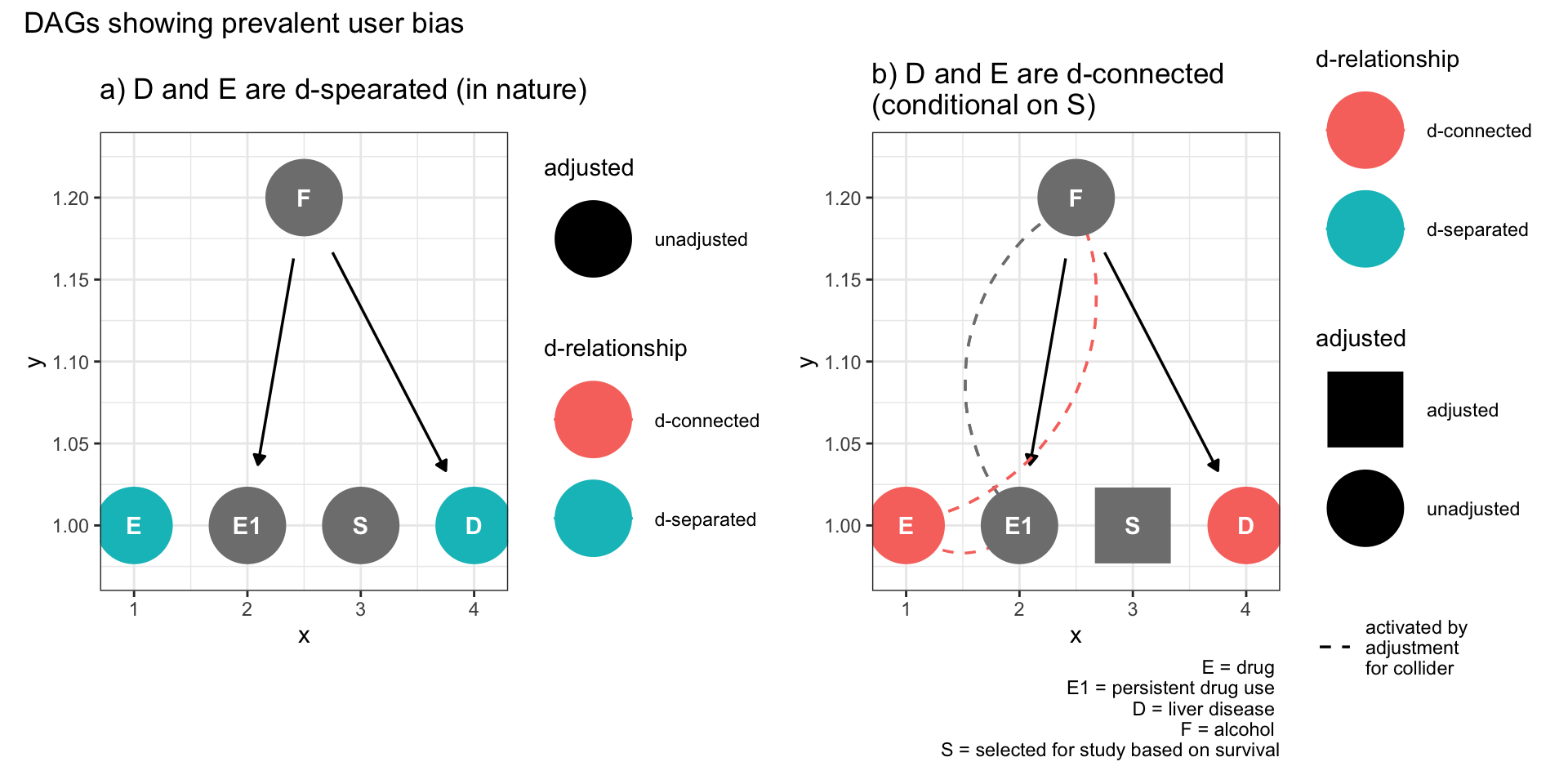
Figure 9.4: Selection bias (prevalent user bias)
This DAG demonstrates an extension of Figure 9.3 that selecting on a descendant of a collider also can open a non-causal path between exposure and outcome.
9.5.3 Index event bias
This bias was introduced in Chapter 7.3. As an example, consider the numerous publications reporting an apparent obesity paradox whereby obesity, a well established cardiac risk factor, is reported to be protective for recurrent myocardial infarctions.
Does anyone honestly believe this to be true? I don’t know of any secondary cardiac prevention clinic which is prescribing weight gain. The following DAG makes it clear that there is no paradox and this observation is entirely compatible with selection bias.
coords <-  list(
  x=c(E=1, F=2.5, D=3, S=2),
  y=c(E=1, F=1.2, D=1, S=1) )

dag <- dagify(D ~ S + F, S ~ F + E, coords = coords)
dag1 <- dag %>% ggdag_drelationship("E", "D") + theme_bw() + ggtitle("a) D and E are d-spearated (in nature)")
dag2 <- dag %>% ggdag_drelationship("E", "D", controlling_for = "S") + theme_bw() + ggtitle("b) D and E are d-connected \n(conditional on S)") +
  labs(caption = "E = age \nD = dementia \nF = smoking \nS = selected for study based on survival of initial event")

dag1 + dag2 +
plot_annotation(title = 'DAGs showing index bias') 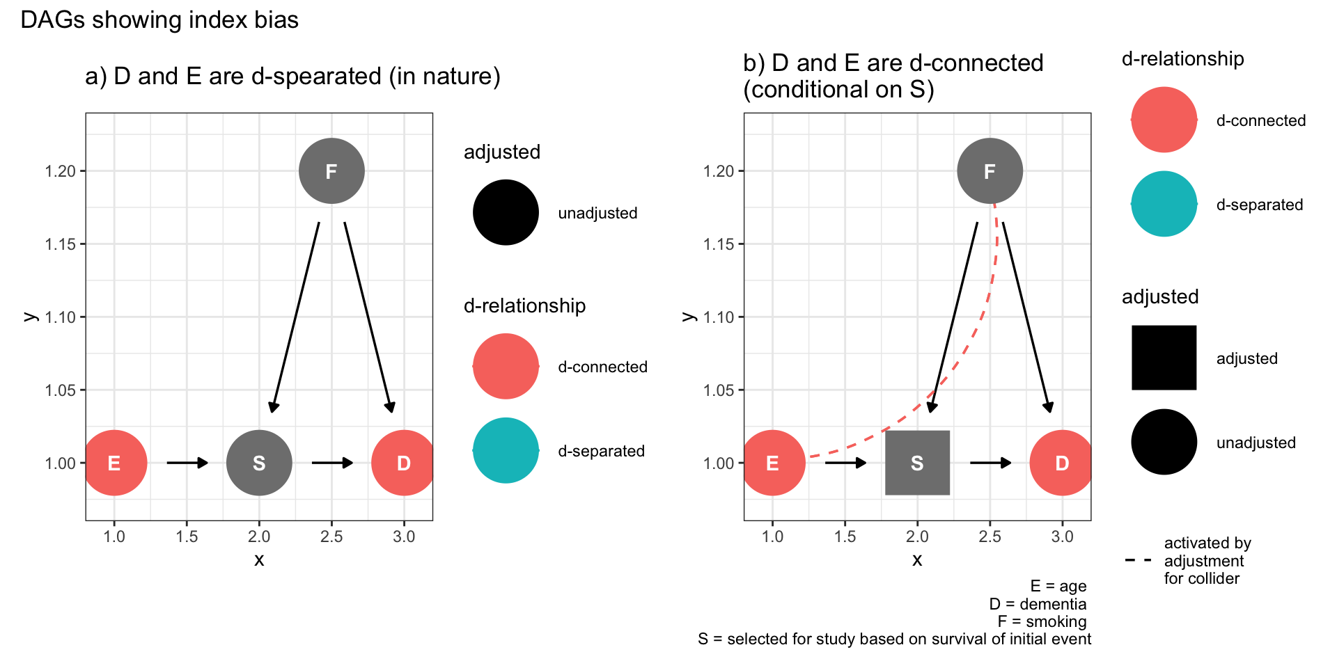
Figure 9.5: Selection bias (index event bias)
The left hand Figure shows that the effect of obesity on recurrent cardiac outcomes (D) is mediated by survival of the first cardiac event (S). On the right, we see that selecting the survivors will create a backdoor pathway between obesity and other variables that effect both initial survival and recurrent events that can account for the observed negative (protective) association. Other cardiovascular “paradoxes” of reduced recurrent events among smokers and those without aspirin are most likely explained by the same selection bias (collidor stratification bias).
Most amazingly, this bias even has a dose response quality. Consider this JAMA publication where among survivors of an initial myocardial infarction, the risk of mortality progressively increased as the number of risk factors decreased!
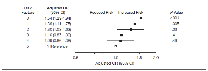
Figure 3.6: Mortality according to risk factors among survivors of an initial MI
Apparently our secondary preventive clinics should not only encourage weight gain but also more smoking, less physical activity and increased cholesterol consumption! Alternatively, we might conclude that this paper falls into the category of false findings discussed in Chapter 5.5.
9.6 Immortal time bias
Immortal time refers to a period of follow-up during which, by design, death or the study outcome cannot occur. This is a frequent problem in observational pharmacoepidemiology studies and is often due to selection bias, although we will see in the next section that misclassification can also explain this bias.
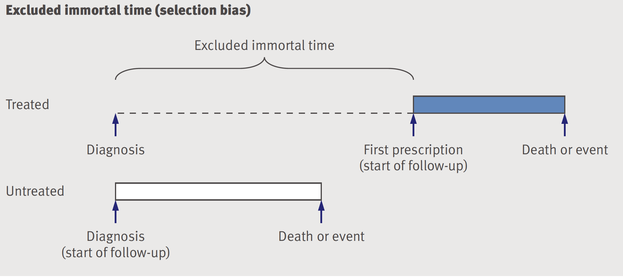
Figure 9.6: Excluded immortal time -selection bias
The issue arises from failure to align eligibility, exposure and follow-up times(Hernan et al. 2016).
While most researchers and readers are well aware of confounding as a potential bias in pharmacoepidemiology studies, it is less well appreciated that the magnitude of immortal time bias is often substantially greater. This is unsurprising for at least three reasons
although many observational studies have unmeasured confounders, like smoking history, obesity or socioeconomic status, the evidence that physicians preferential prescribe as a function of those variables is far from definitive
the smount of excluded time may be substantial and this will leads to a greatly inflated protective effect for the studies drug and
it is established that postive results are easier to publish
9.7 Concluding remarks for selection bias
In an ideal world, selection bias would be avoided at the design or data collection stage but real world realities often make that, at least partially, impossible. As shown above, DAGs can help as a first step to identify possible sources of selection bias. Detailed collection of all variables associated with sample selection and outcomes can help mitigate selection bias. Designing observational studies to emulate RCTs will also help minimize selection (and other) biases. Possible analytical solutions may include complete case analyses, multiple imputation, and inverse probability weighting(Smith 2020).