Chapter 10 Misclassification
10.0.1 R packages required for this chapter
library(knitr)
library(tidyverse)
library(epiR)
library(episensr)
10.1 Introduction
Misclassification is defined as the erroneous classification of an individual, a value or an attribute into a category other than that to which it should be assigned. Misclassification may be considered a measurement error and is also known as information or observational bias.
Misclassification can occur with regards to exposure status, outcome or both and may occur due to flawed definitions or flawed data collection. In case-control designs, misclassification is most often of exposure and can be differential since exposure is measured after outcome. In cohort studies, misclassification of exposure is more likely to nondifferential due to its generally prospective measurement. Misclassification can also occur in RCTs and in this situation is often categorized as detection bias.
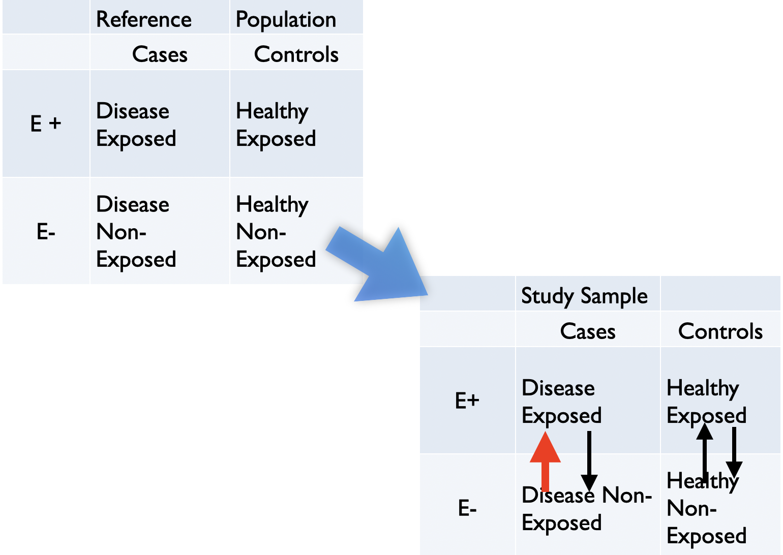
Figure 6.7: Most common misclassification in case control study
Figure 6.7 is typical of recall bias whereby patients with the outcome exhibit increased awareness for exposure compared to the controls. One potential solution for minimizing recall bias is to validate self-reports with historical or current administrative records, if possible.
10.2 Immortal time bias
As discussed in section 9.6, immortal time bias has two potential components, selection bias and a misclassifciation bias as shown in the following figure.
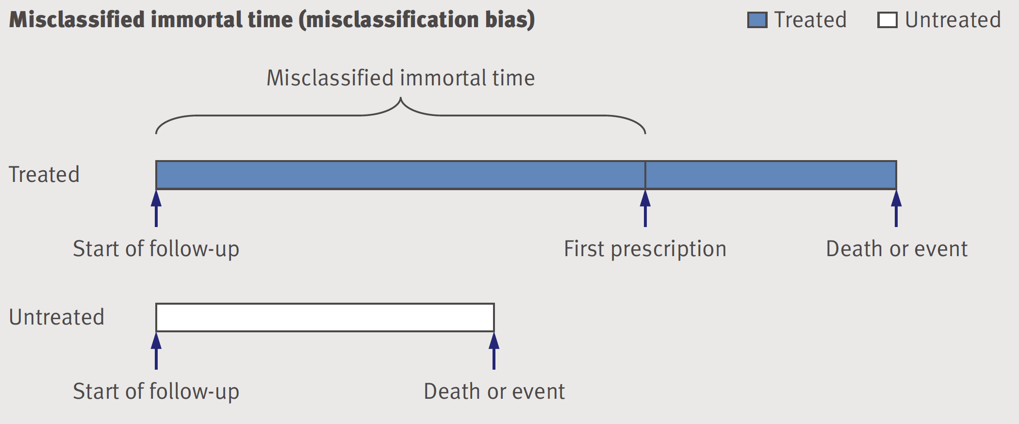
Figure 9.6: Misclassified immortal time - misclassification bias
The time until the drug is prescribed is considered immortal because by definition individuals who end up in the treated or exposed group have to survive without an event until the treatment definition is fulfilled. If they have an event before they are automatically considered to be in the untreated or unexposed group. Whether this period of immortality is treated as misclassification or excluded, the result is bias. One of the advantages of the proposed “emulate target trials” approach for the design of observational studies is to avoid this bias(Hernan et al. 2016).
Immortal time bias example
Levesque and colleagues (Levesque et al. 2010) provide an excellent example of immortal time bias with a reanalysis of a statin study that reported a 26% reduction in the risk of diabetes progression, defined as the need to begin insulin therapy, with one year or more of statin treatment (adjusted hazard ratio 0.74, 95% CI 0.56 to 0.97). Rather than using the original fixed time analysis which allocated all time before drug exposure to the treated group, Levesque perfeormed a time dependent analysis where person days of follow-up were classified as untreated until the study defined one year of statin use definition was met, and as treated thereafter. In fact this time time dependent analysis avoided 3 immortal time periods that were present in the original analysis; 1) 6 months statin free period 2) time from until first prescription was given 3) 1 year of statin prescription time.
This immortal time accounted for 68% of total follow-up time allocated to statin users leading to a spuriously low event rate. The corrected time dependent analysis which avoids the immortal time showed that statin use was associated with an increased risk of progression to insulin, (HR 1.97, 95% CI 1.53 to 2.52). Of course this association is not cauisal and likely confounded by indication as those with diabetes progression are more likley to have heart disease, a strong indication for statins.
Interestingly, Levesque further demonstrated that by using the same biased immortal time design they could show a benefit of decreased diabetes progression with NSAIDs and gastric protection medications, two drug classes with no known effect on diabetes. Finally, the larger the amount of immortal time, the larger the bias and as mentioned previously this may lead to magnitudes of bias far exceeding those of the more commonly recognized confounding bias.
10.3 Medical surveillance bias
When thinking about misclassification or measurement error, it is often helpful to use the framework of sensitivity and specificity (i.e., similar to diagnostic tests). Recall
Sensitivity: Proportion of all truly exposed individuals correctly classified by the study.
Specificity: Proportion of all truly unexposed individuals correctly classified by the study.
This can be helpful as the type of misclassification can be based on the notions of sensitivity and specificity:
Non-differential: Sensitivity and specificity of exposure ascertainment are the same in cases and controls -> bias to the null (usually, if only 2 categories and no other biases)
Differential: Sensitivity or specificity of exposure ascertainment differs between cases and controls -> can’t predict bias direction
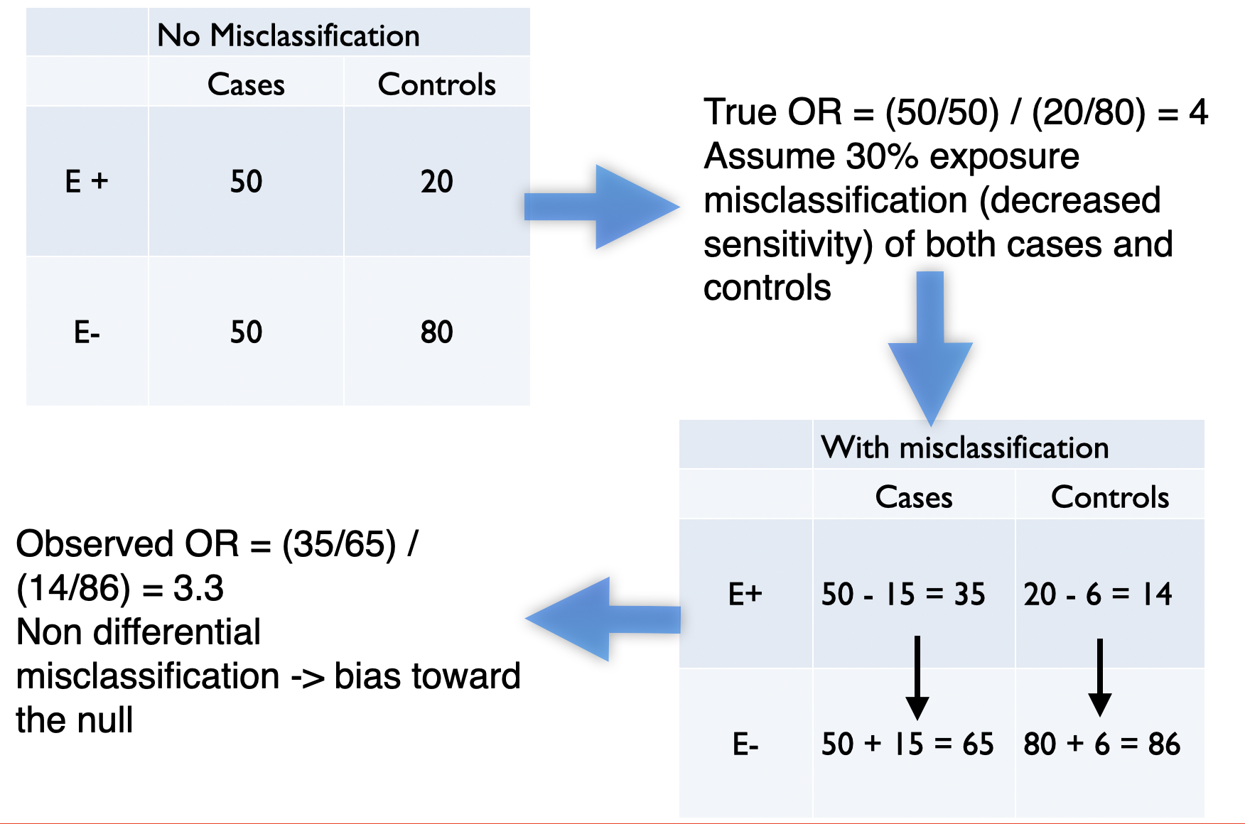
Figure 10.1: Example of non-differential misclassification
10.4 Quantitative bias analysis (QBA)
Very often study biases whether selection, confounding or misclassification bias, are only evaluated qualitatively and not quantitatively. Lash and colleagues have written a book that addresses the issue of quantitative bias analysis(Lash TL 2009) and provide Excel sheets to perform these analyses. Of course, there exists a R package, episensr that performs these calculations. These sensitivity analyses attempt to quantify the direction, magnitude, and uncertainty of the bias affecting an observed effect estimate of association.
Misclassification example using R
A Mayo Clinic study(Hasin et al. 2013) reported that patients who develop heart failure after myocardial infarction have an increased risk of an incident cancer diagnosis. While the authors performed a time to event analysis for this example we will only compare the proportions of those with and without heart failure who develop cancer, since we do not have access to the full dataset. There were 28 incident cancers among the 228 patients with heart failure and 70 cases among the 853 patients without heart failure (OR = 1.5).
dat <- matrix(c(28,70,200,783), nrow=2, ncol=2, byrow=TRUE)
rownames(dat) <- c("Cases", "Controls")
colnames(dat) <- c("Exposed","Unexposed")
dat
## Exposed Unexposed
## Cases 28 70
## Controls 200 783epiR::epi.2by2(dat)## Outcome + Outcome - Total Inc risk * Odds
## Exposed + 28 70 98 28.6 0.400
## Exposed - 200 783 983 20.3 0.255
## Total 228 853 1081 21.1 0.267
##
## Point estimates and 95% CIs:
## -------------------------------------------------------------------
## Inc risk ratio 1.40 (1.00, 1.97)
## Odds ratio 1.57 (0.98, 2.49)
## Attrib risk * 8.23 (-1.07, 17.52)
## Attrib risk in population * 0.75 (-2.75, 4.25)
## Attrib fraction in exposed (%) 28.79 (0.29, 49.14)
## Attrib fraction in population (%) 3.54 (-0.59, 7.49)
## -------------------------------------------------------------------
## Test that OR = 1: chi2(1) = 3.623 Pr>chi2 = 0.06
## Wald confidence limits
## CI: confidence interval
## * Outcomes per 100 population unitsNow the patients with heart failure were followed regularly at the Mayo clinic while the non heart failure patients were followed in the community. It seems quite reasonable to assume that the sensitivity to detect the exposure (cancer diagnosis) among the heart failure cases followed at the Mayo Clinic is greater than that for detecting cancer among community control.
It may be reasonable to assume that sensitivity to detect cancer in the Mayo Clinic patients = 0.9 while in the community it = 0.8. While we could perform the calculations by hand as in section 10.1, this can be done using the episensr package and misclassification function to test the robustness of the original conclusion. Details about the package with vignettes can be found with help(package="episensr"). While we are demonstrating the utiliyu of this package for misclassification, similar functions selection and confounders exist to correct for selection bias and residual confounding.
out <- misclassification(dat, bias_parms=c(.9,.8,1,1), type="outcome")
out## --Observed data--
## Outcome: Cases
## Comparing: Exposed vs. Unexposed
##
##          Exposed Unexposed
## Cases         28        70
## Controls     200       783
##
## 2.5% 97.5%
## Observed Relative Risk: 1.4965 0.9900 2.2621
## Observed Odds Ratio: 1.5660 0.9837 2.4930
## ---
##
## Misclassification Bias Corrected Relative Risk: 1.330
## Misclassification Bias Corrected Odds Ratio: 1.382print("Corrected Table")## [1] "Corrected Table"out$corr.data## Exposed Unexposed
## Cases 31.11 87.5
## Controls 196.89 765.5As expected, correcting for the bias has moved the result towards the null and there is no longer any signal suggesting an increased cancer risk among patients who develop heart failure (OR 1.4, 95%CI 0.8 - 2.2). To further investigate this sensitivity analysis, one could perform a probability sensitivity analysis using the probsens function. For example, rather than assuming fixed sensitivities for exposure among cases and controls one could sample from a probability distribution. For example, assume normal distributions with a sensitivity range of 0.85 - 0.95 and 0.7 - 0.9 for cases and controls, respectively,
probsens(dat,
         type = "exposure",
         reps = 20000,
         seca.parms = list("uniform", c(.85, .95)),
         seexp.parms = list("uniform", c(.7, .9)),
         spca.parms = list("uniform", c(.99, 1)),
         spexp.parms = list("uniform", c(.99, 1)),
         corr.se = .8,
         corr.sp = .8)
## --Observed data--
## Outcome: Cases
## Comparing: Exposed vs. Unexposed
##
## Exposed Unexposed
## Cases 28 70
## Controls 200 783
##
## 2.5% 97.5%
## Observed Relative Risk: 1.4965 0.9900 2.2621
## Observed Odds Ratio: 1.5660 0.9837 2.4930
## ---
## Median 2.5th percentile
## Relative Risk -- systematic error: 1.3328 1.1863
## Odds Ratio -- systematic error: 1.3745 1.2075
## Relative Risk -- systematic and random error: 1.3274 0.8564
## Odds Ratio -- systematic and random error: 1.3682 0.8360
## 97.5th percentile
## Relative Risk -- systematic error: 1.4758
## Odds Ratio -- systematic error: 1.5408
## Relative Risk -- systematic and random error: 2.0407
## Odds Ratio -- systematic and random error: 2.2195It can be appreciated that using a wide distribution of sensitivities, that there is no robust signal for increased cancers among those with heart failure (OR 1.4, 95%CI 0.8 - 2.2).
Note we are not implying quantitative bias analysis provides the exact unbiased answer but it does plainly show the lack of robustness of the original conclusions to a quite reasonable series of sensitivity analyses. QBA calls into question the rather definitive conclusion advanced by the authors “Patients who develop HF after MI have an increased risk of cancer.”