4.1 Sample regression line

• Let consider an hypothetical example where linear dependence between consumption and income on weekly basis is analyzed in a population of $60$ households. Households are divided into $10$ groups with the same level of income as presented in table 4.1.

TABLE 4.1: Weekly consumption of $60$ households with respect to income level

Income ($X$)								$E(Y$|$X)$
80	55	60	65	70	75			65
100	65	70	74	80	85	88		77
120	79	84	90	94	98			89
140	80	93	95	103	108	113	115	101
160	102	107	110	116	118	125		113
180	110	115	120	130	135	140		125
200	120	136	140	144	145			137
220	135	137	140	152	157	160	162	149
240	137	145	155	165	175	189		161
260	150	152	175	178	180	185	191	173

• An average weekly consumption is given by the income level, i.e. the conditional mean (we often say conditional expectation) is a linear function of variable $X$

$$\begin{equation} E(Y|X)=\beta_0+\beta_1X \tag{4.2} \end{equation}$$

• Inserting values from the first and the last column of table 4.1 in equation (4.2) we get

$$\begin{align} 65&=\beta_0+\beta_1 80 \\ 77&=\beta_0+\beta_1 100 \\ ~~~~~~~\vdots \\ 173&=\beta_0+\beta_1 260 \\ \tag{4.3} \end{align}$$

• From any two equations of the system (4.3) it’s easy to find two population parameters

$$\begin{equation} \beta_0=17~~~~~~~~\beta_1=0.6 \end{equation}$$

• Conditional expectations are therefore easily computed for each level of income when population parameters are known

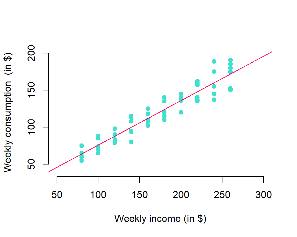
FIGURE 4.1: Population regression line

• Regression line passes through the conditional expectations of variable $Y$ for every level of income $X$

• However, weekly consumption for every household individually $y_i$ differs from the conditional expectation

$$\begin{equation} y_i-E(Y|x_i)=u_i \tag{4.4} \end{equation}$$

• Finally, population regression line is

$$\begin{equation} y_i=\underbrace{\beta_0+\beta_1x_i}_{E(Y|x_i)}+u_i \tag{4.5} \end{equation}$$

• Disturbances $u_i$ are error terms which represent random variables with zero conditional mean for every level of income

$$\begin{equation} E(u|x_i)=0 \tag{4.6} \end{equation}$$

• Condition (4.6) indicates that variable $X$ does not give us any information about error term $u$, i.e. variables $X$ and $u$ are independent

• Population is often finite but unknown or infinite, so the error terms $u_i$ are also uknown as well as parameters $\beta_0$ and $\beta_1$

• Parameters and error terms can be estimated from the sample and thus a sample regression line is

$$\begin{equation} y_i=\underbrace{\hat{\beta}_0+\hat{\beta}_1 x_i}_{\hat{y}_i}+\hat{u}_i \tag{4.7} \end{equation}$$

• Different random samples can be chosen when selecting one household from each group of income level

TABLE 4.2: Two random samples of households with respect to income and consumption

$x_i$ $y_i$ 80 70 100 65 120 90 140 95 160 110 180 115 200 120 220 140 240 155 260 150

$x_i$ $y_i$ 80 60 100 80 120 79 140 108 160 116 180 120 200 144 220 152 240 145 260 178

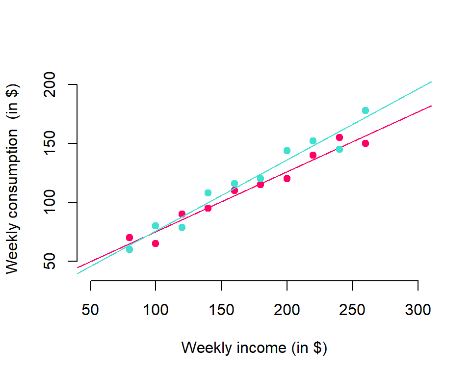
FIGURE 4.2: Two sample regression lines

• Selection of simple random sample requires that error terms are identically distributed (with zero mean and constant variance) and independently distributed (zero covariances)

• Estimated error terms are called residuals and usually denoted as $\hat{u}_i$

• One residual is the difference between the actual value $y_i$ observed from the sample and the fitted or estimated value $\hat{y}_i$ on regression line