Lecture 1 Introduction

1.1 Why mathematical models?

Mathematical models are pervasive in biology. This may not be obvious to undergraduate students because during secondary education mathematical models do not usually feature in the biology curriculum. Whereas mathematics is understood to be an integral part of physics, biology is expected by many to be “maths-free”. This is an unfortunate misconception, as mathematical models feature heavily in virtually all areas of biology. In some areas (such as ecology, epidemiology and evolution), mathematical models have always been important whereas in others they have become central only during the last decades. According to Otto & Day (Otto and Day 2007), 35% of articles published in the journals Ecology and Evolution “reported predictions or results obtained from mathematical models”. (This does not include statistical models!) There are journals devoted entirely to mathematical modelling in biology (e.g., the Journal of Theoretical Biology or PLOS Computational Biology), there are many articles that only report modelling results, and many experimental and empirical articles that also include some modelling results.

Models can serve at least two purposes. First, models can be used to make concrete, quantitative predictions about the future. This is probably what most people would associate with the term ‘mathematical model’. Predictive models seek to answer questions such as: how will climate change affect the abundance of koalas in southern Queensland? How many people are expected to die in the next outbreak of Ebola? How early does one need to start treatment with a certain new antibiotic to avoid the formation of mutant bacteria that are resistant to this antibiotic? Not surprisingly, predictive models require much information about the biological system on which predictions are to be made. Those models tend to be very complex, involving many variables and parameters (see below for definitions of these terms).

Second, there are ‘proof-of-concept’ models. These are models that are studied in order to obtain a general understanding of a type of biological system. Often, the model also helps to assess verbal arguments whose validity is not clear without formalisation (Servedio et al. 2014). For example, ‘proof-of-concept’ models could address questions such as: are complex ecosystems comprising many species more robust towards extinction than simpler ecosystems? Can vaccination of only a subset of a population drive a disease to extinction? Do new beneficial mutations spread faster in well-mixed populations or in populations that are divided into many small subpopulations? Proof-of-concept models are often comparatively simple by design, as they are stripped of everything that is tangential to the problem and go right to the core of the research question. Due to their simplicity, we will mostly deal with such ‘proof-of-concept’ models, but the methods used to study them are the same as for the more complicated predictive models.

1.2 What are mathematical models?

There are quite a few different types of mathematical models. You’ve already encountered many statistical models in the first module of this course. Other models are optimisation models that ask what values of one or several variables need to take so that another variable that depends on them is maximised or minimised. Game theory models that are frequently used in behavioural ecology also belong in this class of models.

Here, we will exclusively deal with another large class of models: dynamical systems. For this reason, we will also use the terms “dynamical system” and “mathematical model” interchangeably throughout these lecture notes. Dynamical systems are models in which one or several variables change through time according to certain rules. Examples that we will frequently encounter include ecological models for how the size of a population changes through time, epidemiological models for how the prevalence of a disease within a host population changes through time, and evolutionary models for how the frequency of a gene changes through time. However, it is important to stress that these models are extremely general: exactly the same modelling techniques that we will cover in this course can also be used in physics (e.g., change in the numbers of different types of atoms during nuclear fusion), chemistry (change in number of molecules during chemical reactions), climate science (e.g., change in temperature through time), economics (change in stock prices), linguistics (change in word use through time), and so on. So, the methods you learn in this course are very broadly applicable throughout science and beyond.

A dynamical system is a an equation or a set of equations that specify how one or several variables will change over time. In addition to those variables, most dynamical systems contain parameters. Those are placeholders that can take different values in the model but that don’t change through time. Keep in mind that what is a variable in one model can be a parameter in another. For example, population size is often a key variable in ecological models, but it is usually a parameter in population genetic models where the size of a population is assumed to be constant through time.

For both variables and parameters, single letters (lower or upper case) can be used in the equations. (When you code your model in R or any other programming language, you can also use words.) The choice of which letter to use is arbitrary, but it’s usually a good idea to follow conventions that prior research has established, e.g. by using \(N\) for population size. For parameters (not so much variables), Greek letters are commonly used. You can also use the same letter with different subscripts for similar variables or parameters, e.g. \(N_f\) and \(N_m\) for the numbers of females and males in a population.

A critical feature of all models are the assumptions on which they rest. Assumptions are necessary to produce a model that is simpler than reality. Some assumptions may be uncontroversial and easy to justify, whereas others are strong and may severely limit the applicability of the model. Therefore, for any model, it is important to state the assumptions clearly, to justify why they are made, to bear them in mind when interpreting the results of your model, and for discussing the limitations of that model.

1.3 What types of models for dynamical systems are there?

There are a number of ways in which mathematical models can be classified. Each type of model makes different assumptions, comes with its own distinctive characteristics and needs to be analysed in a specific way. Therefore, choosing a model type that fits well to the particular biological system that we seek to understand is very important.

The three most fundamental classifications are the following:

1) Discrete vs. continuous time. Discrete-time models assume that time proceeds in a step-wise manner. The variables of the model take certain values at these discrete time points but the model does not predict what will happen between two consecutive time points. For example, in a discrete time population model, the size of a population may be predicted for each consecutive year, but it won’t predict more fine-grained changes happening throughout each year. By contrast, continuous-time models assume that time is a real number so that in principle the model will predict how variables change in very small (technically: “infinitesimally” small) time steps. Conceptually speaking, continuous-time models are a little bit harder to understand than discrete-time models. However, from a mathematical point of view, continuous-time models are often easier to analyse and are in general “better behaved”. We will see an example of this later in the course.

2) One vs. more than one variables. This is a straightforward classification according to how many variables there are in the model. Models with a single variable are commonly encountered and important, but most biological systems of interest involve more than one variable that need to be tracked in order to obtain meaningful insights into the system. Not surprisingly, models with only a single variable are easier to analyse than those with multiple variables. For this reason, we will not be able to cover multi-variable models in the same depth as single-variable models in this course.

3) Deterministic vs. stochastic. In a deterministic model, once all parameters and initial conditions are set, the variables change in a mechanical, “predestined” manner, and multiple iterations of the model produce exactly the same outcome. In stochastic models, the variables are random numbers. Each iteration of the model may therefore produces a different outcome. Stochastic models are very important but much more difficult to analyse than deterministic models, so that we will only scratch the surface of such models in this course.

Models falling within all combinations of these three types exist, and we will encounter examples of most of them.

1.4 How does modelling work?

Following Otto & Day (Otto and Day 2007), the process of modelling a biological problem can be broken down into the following seven steps:

Step 1: Formulate the question. Coming up with a research question that is novel, interesting and important is usually hard, but it is an essential first step in any research project (not just modelling). However, this step is beyond the scope of this course and we will confine ourselves to well-known questions.

Step 2: Determine the model ingredients. The most fundamental ingredient of your model are your variables. Think carefully about what variables your model should include and what other quantities that might also change through time that you can ignore. Also think about the range of values that are biologically plausible for your variable(s). Next, choose how time should be represented in your model (discrete or continuous), and whether your model should be deterministic or stochastic. Finally, determine which parameters your model should include. All of these decisions often involve trade-offs between biological realism and tractability of your model. Ideally, your model should capture the key features of your biological system but nothing more. Finding the right balance here is a crucial part of the art of modelling.

Step 3: Describe the model qualitatively. Before writing down any equations it is usually a good idea to make sure you have sufficient clarity about how the model should work. This can be achieved by drawing diagrams, including flow diagrams in models with several variables. We will see many examples of this later in the course.

Step 4: Write down the equations. Now, you should be ready to write down the equations that define your dynamical system. Depending on the type of model, these may be recursion equations, difference equations, differential equations, or equations specifying events in a stochastic model.

Step 5: Analyse the model. It is now time to try and understand how the model behaves. There are many techniques for this and we will encounter some of the most important ones in this module. A good starting point is often to implement the model in a programming language (we will use R) and simulate how the variables change through time for specific parameter values. More systematic analyses include mathematical techniques such as finding equilibria and determining their stability, and computational approaches such as screening the parameter space in a meaningful way.

Step 6: Checks and balances. Often, your initial analyses may reveal mistakes in the model, or identify undesirable features of your model. It is therefore critical to be alert to such problems, check and double-check your equations and make corrections if necessary.

Step 7: Relate the results back to the question. Once you have made sure that your model works and you have obtained a good understanding of the behaviour of your model, it is time to relate these results back to reality. Keeping in mind the assumptions you’ve made, what does your model tell you about how the biological system that you studied should behave? Your model may make interesting predictions that could be the basis of experimental tests or other models that explore these predictions in more detail.

1.5 Exercises

1. Solve the following equations for \(x\):

\[\begin{gathered} 6x-2=7 \qquad \frac{1}{1-x}=x-3 \qquad e^{5-3x}=2 \qquad 5^{x^2}=625 \qquad \ln(x)=2x \end{gathered}\]

2. Draw sketches of the following functions and obtain their derivatives: \[\begin{gathered} f(x)=3x+2 \qquad g(x)=(x-2)(x-5) \qquad h(x)=1+\frac{1}{x-1} \\ k(y)=\frac{1}{10+y} \qquad p(x)=2e^{-x} \qquad q(x)=-3e^{(x+1)^2} \\ x(t)=\frac{5}{1+e^{-t}} \qquad y(x)=\ln(x-1) \qquad z(y)=\ln(\sqrt{y}) \end{gathered}\]

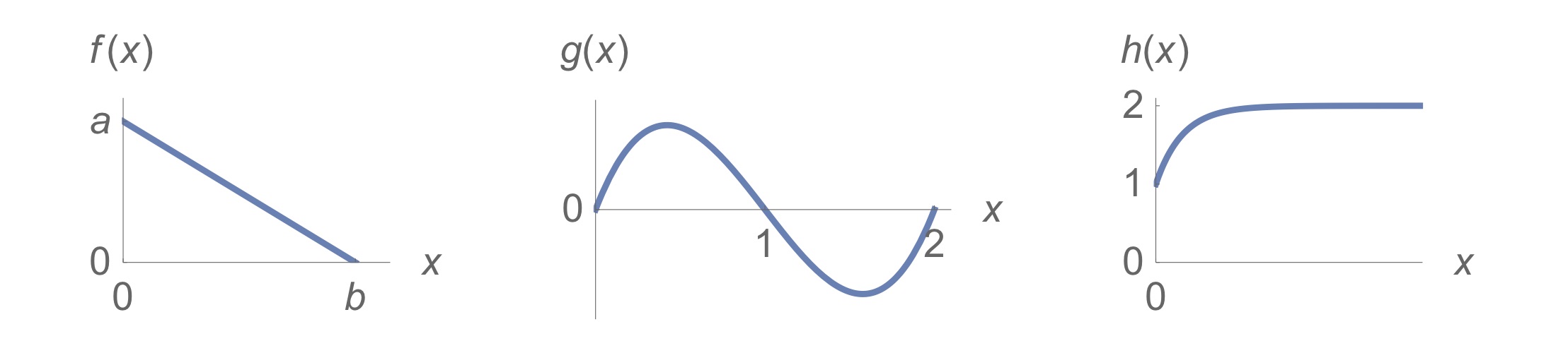
3. Come up with equations that match the following functions:

4. Go to the website of the journal The American Naturalist and choose five research articles from the current tables of contents that catch your attention. Skim those articles and try to answer the following questions for each of them: Does the article contain a mathematical model? If so: what type of model is it, and what are its variables and parameters?

References

Otto, S. P., and T. Day. 2007. A Biologist’s Guide to Mathematical Modeling in Ecology and Evolution. Book. Princeton: Princeton University Press. http://www.loc.gov/catdir/enhancements/fy0704/2006044774-b.html.

Servedio, M. R., Y. Brandvain, S. Dhole, C. L. Fitzpatrick, E. E. Goldberg, C. A. Stern, J. Van Cleve, and D. J. Yeh. 2014. “Not Just a Theory–the Utility of Mathematical Models in Evolutionary Biology.” Journal Article. PLOS Biology 12 (12): e1002017. doi:10.1371/journal.pbio.1002017.