Lecture 4 Continuous-time models in several variables

In this lecture we will extend the one-variable ODE models covered in the last chapter to include more than one variable. We will focus on compartmental epidemiological models of disease spread as examples and appreciate the importance of flow diagrams of these models. We will learn how equilibria of these models can be obtained but we won’t systematically analyse the stability of these equilibria as this requires techniques from multivariate calculus that you may not be familiar with. For an in-depth treatment of compartmental models of disease spread and their applications see the excellent book by Keeling & Rohani (Keeling and Rohani 2008).

4.1 The SI model

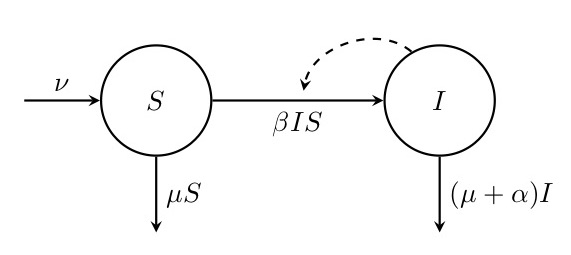
We start by considering one of the simplest epidemiological models in which there are two types of individuals: susceptibles and infecteds. We denote the number of these two types of individuals by \(S\) and \(I\). We assume that susceptibles can become infected by contact with infected individuals and that infected people never recover. Both susceptible and infected individuals die at a per capita mortality rate \(\mu\) (mu). In addition to this natural mortality, infected individuals can also die from the disease at a per capita rate \(\alpha\) (alpha, often referred to as the virulence of a disease). Finally, we assume that new susceptible individuals enter the population at a fixed rate \(\nu\) (nu). These assumptions can be summarised in the flow diagram in Fig. (1).

What we haven’t specified yet is how transmission is going to happen. Intuitively, the per capita rate at which susceptible individuals become infected (technically called the force of infection) should increase with increasing numbers of infected individuals. Here, we go for the simplest out of many different options and assume that the force of infection increases linearly with the number of susceptible individuals at a rate \(\beta\), i.e. the force of infection is equal to \(\beta I(t)\).

We are now in a position to translate the diagram in Fig. (1) into a set of two ODEs:

\[\begin{equation} \tag{4.1} S'(t) = \nu - \beta I(t) S(t) - \mu S(t) \end{equation}\] \[\begin{equation} \tag{4.2} I'(t) = \beta I(t) S(t) - (\mu + \alpha)I(t) \end{equation}\]

These two equations are said to be coupled because the equation for each of the two variables also contains the other variable. Our model is now fully specified (Step 4 in Section 1.4). To analyse this model, we could first try and see how it behaves with specific parameters by solving the equations numerically. We will see how this can be done in R during the practical.

Figure. 1: Flow diagram of the SI model. This diagram shows how the numbers of susceptible (\(S\)) and infected (\(I\)) individuals are assumed to change through time depending on the migration rate \(\nu\), the death rate \(mu\), the transmission rate \(\beta\) and the disease-related mortality \(\alpha\). Solid arrows indicate flow in and out of compartments, and the dashed arrow indicates that \(I\) has an impact on the rate of transition from \(S\) to \(I\).

To gain deeper insights into the general behaviour of our model, we can again derive its equilibria. With more than one variable, a system is said to be in equilibrium if none of its variables exhibit any change in time. Therefore, we need to work out under what conditions \[\begin{equation} \tag{4.3} S'(t)=0 \quad \text{and} \quad I'(t)=0 \end{equation}\]

hold simultaneously. Examining Eq. (4.2) reveals that \(I'(t)=0\) when

\[\begin{equation} \tag{4.4} 0 = I(t) \left(\beta S(t) - \mu - \alpha \right) \end{equation}\]

holds. One solution to this equation is \(I(t)=0\). This makes sense: if there are no infected individuals in the population, there never will be any in the future. We can thus replace \(I(t)\) by \(0\) in Eq. (4.1) and solve the resulting equation

\[\begin{equation} \tag{4.5} 0 = \nu - \mu S(t) \end{equation}\]

for \(S(t)\). This gives us our first equilibrium

\[\begin{equation} \tag{4.6} (\widehat{S_1}, \widehat{I_1}) = \left(\frac{\nu}{\mu}, 0 \right) \end{equation}\]

This equilibrium corresponds to the case when the disease is not present in the population and the number of uninfected individuals has reached a balance between migration and death.

To obtain a second equilibrium, we can assume \(I(t)>0\), which means that the second factor in Eq. (4.4) must be equal to zero. Thus, we can solve

\[\begin{equation} \tag{4.7} 0 = \beta S(t) - \mu - \alpha \end{equation}\]

for \(S(t)\) to yield \(\widehat{S}_2=(\mu+\alpha)/\beta\). Next, we can plug this expression into our equation for \(S'(t)\) (Eq. (4.6)), set it to zero as well and solve for \(I(t)\):

\[\begin{align} S'(t) &= 0 = \nu - \beta I(t) \widehat{S}_2 - \mu \widehat{S}_2 \\ \Leftrightarrow \quad I(t) & = \frac{\nu}{\beta \widehat{S}_2} - \frac{\mu}{\beta} = \frac{\nu}{\beta \frac{(\mu+\alpha)}{\beta}} - \frac{\mu}{\beta} = \frac{\nu}{\mu+\alpha} - \frac{\mu}{\beta}. \tag{4.8} \end{align}\]

This completes the derivation of our second equilibrium,

\[\begin{equation} (\widehat{S_2}, \widehat{I_2}) = \left(\frac{\mu + \alpha}{\beta}, \frac{\nu}{\mu+\alpha} - \frac{\mu}{\beta} \right) \tag{4.9} \end{equation}\]

In order to be biologically meaningful, both \(\widehat{S_2}\) and \(\widehat{I_2}\) must not be negative. \(\widehat{S_2}\) is always positive because \(\mu\), \(\alpha\) and \(\beta\) are all positive rates. However, \(\widehat{I_2}\) is positive only when

\[\begin{equation} \tag{4.10} \frac{\nu}{\mu+\alpha} > \frac{\mu}{\beta}, \end{equation}\]

or when

\[\begin{equation} \tag{4.11} \frac{\beta \nu}{\mu(\mu+\alpha)} = \frac{\beta \widehat{S}_1}{\mu+\alpha} > 1. \end{equation}\]

The left-hand side of inequality (4.11) is called \(R_0\), the basic reproductive number. This number determines whether or not a disease can spread in a population. It can be interpreted as the number of new infections that an infected individual causes in an otherwise uninfected population. Per unit of time, such an individual will cause \(\beta \widehat{S}_1\) new infections because at equilibrium 1 there will be \(\widehat{S}_1\) uninfected individuals. The individual will be able to infect other individuals for a duration of \(1/(\mu + \alpha)\) since it will die at a rate \((\mu + \alpha)\). (Remember that if something happens at a certain rate \(r\), it will take on average \(1/r\) units of time for this to happen.) Multiplying the infection rate per unit of time with the duration of infectivity then gives us \(R_0\). Intuitively, an infected individual must infect more than one new individual over the course of infection for the disease to spread, which is exactly the condition \(R_0>1\) inequality (4.11). It can also be shown that if condition (4.11) holds, the endemic equilibrium \((\widehat{S_2}, \widehat{I_2})\) is always a stable equilibrium and the disease-free equilibrium \((\widehat{S_1}, \widehat{I_1})\) is always unstable, but this is beyond the scope of this course.

4.2 The SIR model

The SI model is only one out of a large number of epidemiological models that differ in the number of compartments as well as the assumptions concerning demography and transmission, amongst others. The most famous of these models is the SIR model. Here, a third class of individuals that have recovered from the disease and are immune to future infections is considered. In the simplest form, this model can be visualised as shown in Fig. (2) and written down by the following corresponding ODE system:

\[\begin{equation} \tag{4.12} S'(t) = -\beta I(t) S(t) \end{equation}\] \[\begin{equation} \tag{4.13} I'(t) = \beta I(t) S(t) - \gamma I(t) \end{equation}\] \[\begin{equation} \tag{4.14} R'(t) = \gamma I(t) \end{equation}\]

Here, \(\beta\) is again the per capita transmission rate and \(\gamma\) is the recovery rate, which means that \(1/\gamma\) can be interpreted as the average infectious period of the disease. For simplicity, we have now ignored any demographic processes, i.e. no new individuals enter the population and there is no death. This situation may be realistic for diseases that spread very rapidly but don’t impose any mortality on their hosts. Of course, demographic processes such as those assumed for the SI model in the previous section can also be incorporated into the SIR model.

Figure. 2: Flow diagram of the SIR model. This diagram shows how the numbers of susceptible (\(S\)), infected (\(I\)) and recovered (\(R\)) individuals are assumed to change through time depending on the transmission rate \(\beta\) and the recovery rate \(\gamma\). Solid arrows indicate flow in and out of compartments, and the dashed arrow indicates that \(I\) has an impact on the rate of transition from \(S\) to \(I\).

We might conjecture that assuming \(I(t)=0\) will again reveal an equilibrium of the model. Indeed, after substituting zero for \(I(t)\) in Equations (4.12) to (4.14), we see that all three equations immediately become zero (\(S'(t)=I'(t)=R'(t)=0\)), independent of what values \(S(t)\) and \(R(t)\) take. This represents a situation that we haven’t encountered before: there are infinitely many equilibria given by all possible values of \(S(t)\) and \(R(t)\) provided that \(I(t)=0\). This is simply because when the population is infection-free, there is nothing left that impacts the number of susceptible or recovered (immune) individuals in the population.

Next, we can ask under what conditions the disease could spread in a population consisting only of susceptible individuals. This means that we need to find out under what conditions \(I'(t) = \beta I(t) S(t) - \gamma I(t) > 0\). Assuming that there are some infected individuals in the population that could start an epidemic, this inequality can be solved to yield

\[\begin{equation} \tag{4.15} \frac{\beta S(t)}{\gamma} >1 \end{equation}\]

This condition reveals an important insight: for the disease to spread, it is not only important that the transmission rate \(\beta\) is high and the recovery rate \(\gamma\) low (so that infected individuals remain infectious for a long time), but there also needs to be a minimum number of susceptible individuals present in the population. By contrast, the number of recovered individuals is completely irrelevant for disease spread. Note that the left-hand side of inequality (4.15) can again be interpreted as the basic reproductive number \(R_0\).

Apart from the infinitely many equilibria that we get when \(I(t)=0\), is there another equilibrium with the disease being present in the population? Reconsidering Equations (4.12) to (4.14), we can see that the answer is no. If we set these three equations to zero and assume \(I(t)>0\), we can divide all three equations by \(I(t)\) so all \(I\)’s disappear and there simply is no solution to the resulting system of equations.

We can now try to make an educated guess about the general behaviour of the model. As we’ve seen, the disease can spread when rare into a population of susceptible individuals if \(R_0=\frac{\beta S(t)}{\gamma}>1\). However, as the disease spreads it does not reach an endemic equilibrium in the population because the equations reveal that no such equilibrium exists. Instead, as the number of susceptible individuals gets depleted more and more, the right-hand side of equation (4.13) becomes smaller and smaller until it eventually becomes negative and, consequently, the number of infected individuals declines until the disease has disappeared from the population. This decline is not necessarily caused by the absence of susceptible individuals but rather by the fact that there are too few susceptibles to sustain the epidemic (see Eq. (4.15)).

library(shiny)
library(deSolve)

plotSIR <- function(beta = 0.0002, gamma = 0.5, S0 = 800, I0 = 10, R0 = 0, 
                    tmax = 100) {
    times <- seq(0, tmax, 1)
    
    parameters = c(beta = beta, gamma = gamma)
    
    iniState <- c(S = S0, I = I0, R = R0)
    
    solution <- ode(iniState, times, SIRmodel, parameters)
    
    par(mar = c(5, 5, 0, 0), oma = c(0, 0, 1, 1), mgp = c(2.5, 1, 0), xpd = T)
    plot(NA, xlab = "Time", ylab = "Number of individuals", ylim = c(0, 1200), 
         xlim = c(0, tmax), cex.lab = 2)
    lines(x = solution[, "time"], y = solution[, "S"], col = "black", lwd = 3)
    lines(x = solution[, "time"], y = solution[, "I"], col = "red", lwd = 3)
    lines(x = solution[, "time"], y = solution[, "R"], col = "blue", lwd = 3)
    
    legend(x = 'top', y = 1100, legend = c("S", "I", "R"), 
           col = c("black", "red", "blue"), lwd = 3, horiz = T, bty = "n", cex = 2) 
}

SIRmodel <- function(times, state, parameters) {
    with (as.list(c(state, parameters)), {
        dS <- - beta * I * S 
        dI <- beta * I * S - gamma * I
        dR <- gamma * I
        return(list(c(dS, dI, dR)))
    })
}

app <- shinyApp(
    ui = fluidPage(
        titlePanel("SIR Model"),
   
        sidebarLayout(
            sidebarPanel(      
                sliderInput("transmission", "Transmission Rate:",
                    min = 0, max = 0.001,
                    value = 0.02, step = 0.00001),
                 
                sliderInput("recovery", "Recovery Rate:",
                    min = 0, max = 1,
                    value = 0.5, step = 0.001),
                 
                sliderInput("S0", "Initial Susceptible Individuals:",
                    min = 100, max = 1000,
                    value = 800, step = 100),
                 
                sliderInput("I0", "Initial Infected Individuals:",
                    min = 1, max = 100,
                    value = 10, step = 1),
                 
                sliderInput("tmax", "Time:",
                    min = 100, max = 1000,
                    value = 200, step = 100)
     
            ),
    
            mainPanel(
                plotOutput("plot")
            ),
    
            "left"
        )
    ),

    server = function(input, output) {
        output$plot <- renderPlot({
            plotSIR(beta = input$transmission, gamma = input$recovery, S0 = input$S0, 
                    I0 = input$I0, R0 = 0, tmax = input$tmax)
        })
    }
)

runApp(app)

4.3 Population dynamics with two species

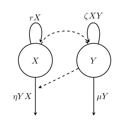
As a final example, let us consider a famous ODE model with two variables from the field of ecology, the Lotka-Volterra model. Here, we follow the population dynamics of two interacting species: prey and predators. Figure (3) illustrates this model and the corresponding equations are:

\[\begin{equation} \tag{4.16} X'(t) = r X(t) - \eta Y(t) X(t) \end{equation}\] \[\begin{equation} \tag{4.17} Y'(t) = \zeta X(t) Y(t) - \mu Y(t) \end{equation}\]

Here, \(X\) is the number of prey and \(Y\) is the number of predator individuals.

Figure. 3: Diagram of the Lotka-Volterra model. In this model, prey individuals (\(X\)) reproduce at a constant per capita rate but die at a rate that is proportional to the number of predators (\(Y\)). Predators reproduce at a per capita rate that is proportional to the number of prey individuals and die at a constant per capita rate.

We can again find the equlibria of this model by setting the right-hand side of Equations (4.16) and (4.17) to zero, i.e. by simultaneously solving

\[\begin{align} 0 & = r X(t) - \eta Y(t) X(t) = X(t) \left( r - \eta Y(t) \right) \\ 0 & = \zeta X(t) Y(t) - \mu Y(t) = Y(t) \left( \zeta X(t) - \mu \right) \tag{4.18} \end{align}\]

for \(X(t)\) and \(Y(t)\). It can be seen that one solution to this system of equations is the equlibrium \((\widehat{X_1}, \widehat{Y_1})=(0,0)\), i.e. the absence of both prey and predators. The second equilibrium can be found by solving

\[\begin{align} (\#eq:CTMSV_LVfindingEquiC) 0 = r - \eta Y(t) \quad \text{and} \quad 0 =\zeta X(t) - \mu, \tag{4.19} \end{align}\]

which gives \((\widehat{X}_2, \widehat{Y_2})=(\frac{\mu}{\zeta}, \frac{r}{\eta})\).

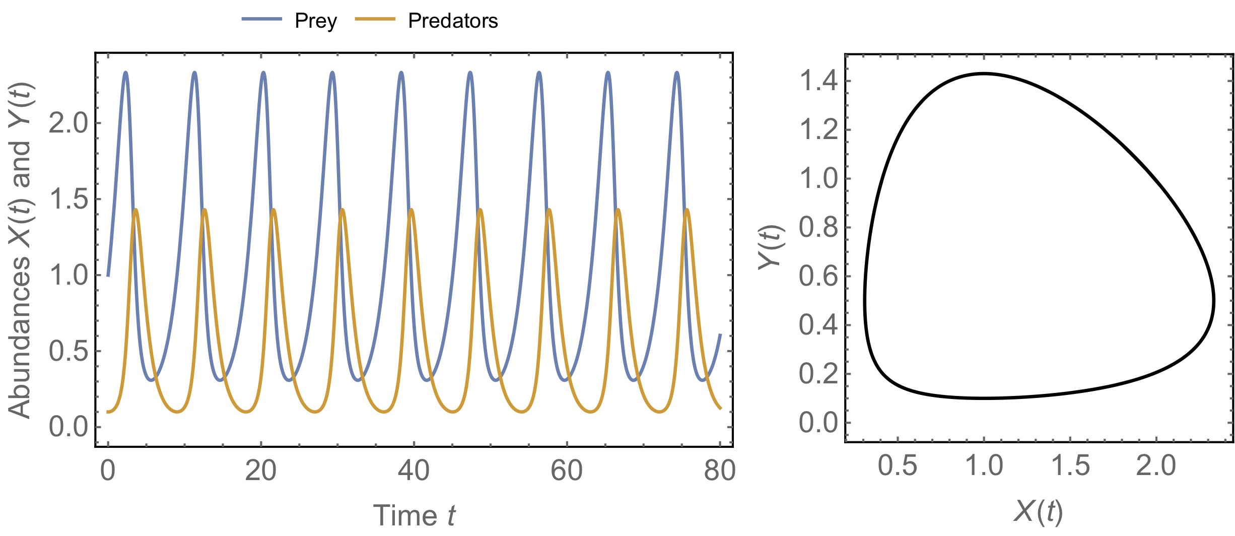
It turns out (but we won’t demonstrate this here) that both of these equilibria are unstable. In the long run, as illustrated in Fig. (4), the system classically exhibits oscillations in the numbers of both species that are not dampened.

Figure. 4: Example dynamics of the Lotka-Volterra model for predator-prey interactions. The left panel shows the oscillatory dynamics of prey and predators through time. The right panel is a phase diagram, which is an alternative way of representing the same dynamics. Time is not explicitly shown but instead the plot shows the corresponding values of the two variables. In this example, the system moves counterclockwise along the circular shape, indicating non-damped oscillations. Parameters take the values \(r=0.6\), \(\eta=1.2\), \(\zeta=\mu=1\).

4.4 Exercises

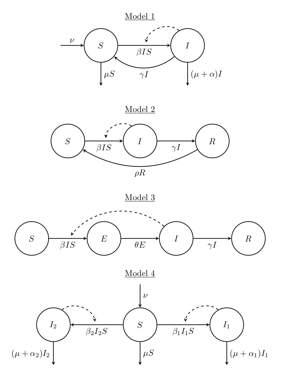
1. Consider the flow diagrams for the following four epidemiological models:

For each of these models,

1. Explain the model in words and say what the variables and parameters might represent,
2. Write down the corresponding ODE system,
3. Determine the equilibria of the system, and
4. Make an educated guess as to how the system will behave.

2. Bacterial species can have complex interactions with each other, for example through the production of toxins that kill other species. Let us assume that there are three bacterial species: Abacter, Bbacter and Cbacter. Each of these species grows at the same rate \(r\) and they compete for the same resources so that logistic growth with a single carrying capacity can be assumed. Abacter produces a toxin that kills Bbacter, and we assume that this happens at a per capita death rate \(\mu\) that is proportional to the number of individuals of Abacter. Bbacter produces a toxin that kills Cbacter in the same manner, and Cbacter produces a toxin that kills Abacter.

1. Produce a diagram for the model described above.
2. Write down the corresponding system of ODEs.
3. Determine the equilibria of the system.
4. What kind of dynamics do you expect to see in this system?

3. The models of population growth covered in Lectures 2 and 3 did not involve any age-structuring within the population. For this exercise, construct a continuous-time mathematical model for an age-structured population with two age-classes: juveniles and adults. Adults reproduce according to the logistic growth assumption, i.e. the rate of reproduction declines linearly with increasing number of adults. Juveniles become adults at a certain rate, and both juveniles and adults die at certain (potentially very different) rates.

1. Make a list of the variables and parameters of the model.
2. Draw a diagram illustrating your model.
3. Write down the corresponding system of ODEs.
4. Determine the equilibria of the system.
5. Can there ever be more adults than juveniles at equilibrium? If so, under what conditions?

References

Keeling, M. J., and P. Rohani. 2008. Modeling Infectious Diseases in Humans and Animals. Book. Princeton: Princeton University Press.