Lecture 2 Discrete-time models in one variable

Conceptually, discrete-time models in one variable are the simplest type of dynamical model, also because understanding them does not require knowledge of any advanced mathematical techniques. Starting from the mathematical concept of sequences and recursion functions, we will consider a number of classic models of population growth in this section, including the Fibonacci model, the exponential model and the logistic growth model. We will finish by introducing the important concept of equilibria and how we can determine their stability.

2.1 Sequences and recursions

A good starting point for thinking about discrete-time models are sequences of numbers that follow certain rules. Consider the following examples:

1 -2 4 -8 16 -32
4 8 32 512 131072
4 5 7 10 14 19
2 4 8 7 5 1

Can you guess the underlying rule for these sequences? (Puzzles like this are frequently encountered in IQ tests.) Sometimes, the rules for building series like the examples above can be written down as recursion equations. This means, if the sequence consists of the numbers \(a_0, a_1, a_2, a_3, ...\), a relationship

\[\begin{equation} \tag{2.1} a_{i+1}=f(a_i) \end{equation}\]

holds for all \(i\geq1\). The function \(f\) takes a number as an argument and transforms it to yield the next number in the sequence. Note that \(a_0\), the first element of the sequence, needs to be specified separately because no previous number exists that \(f\) could operate on.

Let’s make this more concrete by looking again at our examples. The recursion equation for Example 1 can be written as

\[\begin{equation} \tag{2.2} a_{i+1}=-2a_i, \end{equation}\]

with \(a_0=1\). Thus, the function \(f\) defining the recursion equation is \(f(x)=-2x\). Try to write down the recursion equations for the other examples. What problems do you encounter?

2.2 Fibonacci population growth

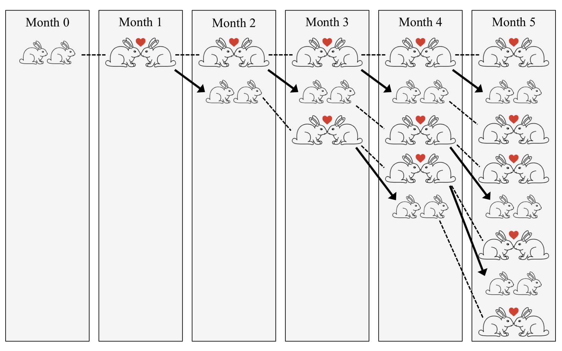Figure. 1: Illustration of the Fibonacci model for population growth. Dashed lines connect identical couples, hearts indicate mating, and arrows indicate offspring.

To see what this all has to do with biological models, we will now swiftly move on to what was perhaps the first model of population growth. This model goes back to Leonardo of Pisa, an Italian mathematician who lived in the late Middle Ages and is better known as Fibonacci. Fibonacci assumed pairs of rabbits that start mating after one month of growth and then indefinitely produce a new couple of baby rabbits each month. So, starting with a newborn couple at time zero, there would still be only one couple after one month. After two months, there would be two couples because the initial couple had reproduced. After three months, there would be three couples because the initial couple had reproduced yet again, but the second couple had not yet reproduced. After four months, there would be five couples because now the first two couples would each produce a new pair of rabbits, and so on (see Fig. (1). In total, this leads to the famous Fibonacci series:

\[\begin{gathered} 1 \quad 1 \quad 2 \quad 3 \quad 5 \quad 8 \quad 13 \quad 21 \quad ... \end{gathered}\]

Close inspection reveals the simple rule for this sequence: each number is the sum of the two previous numbers, and the first two numbers are set to one. Thus, in contrast to Eq. (2.1), we have to go back two numbers in the sequence to obtain a new number. The Fibonacci sequence pops up in many unlikely places in mathematics (e.g., the ratio of two consecutive numbers converges to the Golden ratio), computer science and biology (e.g., plant branching patterns). However, the Fibonacci series is not a particularly good model for population growth because it rests on a number of strong but unrealistic assumptions (which?). Therefore, let us now consider some other models that are more commonly used in population ecology.

2.3 Exponential population growth

Consider a population of asexually reproducing individuals. In each generation, each individual produces on average \(a\) offspring individuals, following which the entire parental generation dies. This assumption is often referred to as “non-overlapping generations” and is met in many plant and animal species. The population is completely homogeneous (no sexes, no age classes, no geographic structure). If we denote by \(N_t\) the number of individuals in generation \(t\), we can write the recursion equation for this model as

\[\begin{equation} \tag{2.3} N_{t+1}=a N_t \end{equation}\]

(As a side note, this is also what happens to money in a bank account with a constant interest rate. To predict how your fortune multiplies if you leave it be, you can simply set \(a\) to one plus the interest rate per time unit.)

To see how this model behaves, let’s just write down the population sizes resulting from this model for a number of generations. Starting with an arbitrarily chosen initial population size \(N_0\) we get

\[\begin{align} N_1 &= a N_0 \\ N_2 &= a N_1=a (a N_0)=a^2 N_0 \\ N_3 &= a N_2=a (a^2 N_0)=a^3 N_0 \\ N_4 &= a N_3=a (a^3 N_0)=a^4 N_0 \tag{2.4} \end{align}\] It is becoming obvious now that in general, \[\begin{equation} \tag{2.5} N_{t}=a^t N_0 \end{equation}\]

So, if we want to know what our model predicts for any generation, we can simply use Eq. (2.5) rather than first calculating all the previous generations. Eq. (2.5) can be understood as the solution of the recursion equation. Unfortunately, such a solution can usually be found only for very simple models.

What then does our solution tell us about the long-term behaviour of our model population? Eq. (2.5) represents an exponential relationship. When \(a<1\), \(a^t\) becomes very small (approaches zero) for large \(t\), so that we would expect the population to go extinct. This makes sense: when each individual produces less than one offspring individual on average, the population cannot be sustained. Conversely, when \(a>1\), the population will grow. More precisely, the population will very quickly reach astronomical numbers and keep growing indefinitely. This is again not very realistic, so that we will next consider the logistic growth model, an extension of the exponential model in which population growth is bounded.

2.4 Logistic population growth

We will now assume that the number of surviving offspring that an individual produces isn’t constant but instead decreases with increasing population size:

\[\begin{equation} \tag{2.6} a=a(N)=b\left(1-\frac{N}{M}\right) \end{equation}\]

When the population is very small (\(N\approx 0\)), this is about equal to the baseline offspring number \(b\), which is the maximum number of offspring that individuals can produce in the absence of any competition with other individuals. As \(N\) increases towards \(M\), \(a\) decreases towards zero, reflecting increasing competition for resources. When the population size is \(M\), competition is so fierce that \(a\) becomes zero and the entire population collapses. Substituting this new, population size-dependent offspring number for the constant \(a\) in Eq. (2.6) yields the logistic growth equation

\[\begin{equation} \tag{2.7} N_{t+1}=b\left(1-\frac{N_t}{M}\right) N_t. \end{equation}\]

We could analyse Eq. (2.7) directly, but it is more useful and common to first transform this equation into a simpler but equivalent version. To this end, we define as a new variable \(x\) the population size relative to the maximum possible population size \(M\), i.e. \(x:=N/M\). With this new variable, we can re-write Eq. (2.7) as

\[\begin{equation} \tag{2.8} x_{t+1}=b(1-x_t)x_t, \end{equation}\]

The nice thing about this transformed equation is that it has only a single parameter \(b\) because the parameter \(M\) has disappeared in the process of normalisation. Try to verify that Eq. (2.8) is indeed equivalent to Eq. (2.7)!

Note that the maximum possible value of \(b\) that leads to meaningful results is \(b=4\). This is because for \(b>4\), relative population sizes above one can arise, which would then lead to negative population sizes in the next generation. This illustrates a major limitation of the model that needs to be kept in mind.

Let us now try to understand how our logistic growth model behaves. Looking at Eq. (2.8) you might expect that the model is just as easy to solve as the exponential model and that the model will always behave in an easily predictable manner. However, the simplicity of Eq. (2.8) is deceptive. In fact, no general solution can be found and the model is famous for producing very rich dynamics that may involve cyclic or even chaotic behaviour! Exploring this in detail is beyond the scope of this course, but we can shed some light on the model by using two important techniques: the graphical method and the analysis of the model’s equilibria.

To explore the dynamics of the logistic model of population growth to the exponential growth model you can run the following app:

library(shiny)

#source("Apps/ExpLogApp/plotGrowth.R")

plotExp <-  function(rate = 2, size = 10) {
  time <- seq(0, 20, 0.1)
  
  par(mar = c(5, 5, 0, 0), oma = c(0, 0, 1, 1), mgp = c(2.5, 1, 0))
  plot(x = time, y = rate^time*size, type = "l", col = "red", 
        ylab = "Population Size", xlab = "Time", cex.lab = 2, lwd = 2)
}
 
plotLog <-  function(rate = 2, size = 10, maxsize = 40) {
  time <- seq(0, 100, 1)

  y <- vector(length = length(time))
  y[1] <- size/maxsize
  for (i in 2:length(time)) {
    y[i] <- rate * (1 - y[i - 1]) * y[i - 1]
  }
  par(mar = c(5, 5, 0, 0), oma = c(0, 0, 1, 1), mgp = c(2.5, 1, 0))
  plot(x = time, y = y, ylim = c(0, 1), type = "l", col = "red", 
        ylab = "Pop Relative to Maximum", xlab = "Time", cex.lab = 2, lwd = 2)
}

app <- shinyApp(
    ui = fluidPage(
        titlePanel("Exponential vs. Logistic Growth"),
  
        tabsetPanel(
            tabPanel("Exponential", fluid = TRUE,
                sidebarLayout(
                    sidebarPanel(      
                        sliderInput("rate1", "Growth Rate:",
                            min = 0.5, max = 4.5,
                            value = 2, step = 0.1),
     
                        sliderInput("size1", "Initial Population Size:",
                            min = 5, max = 50, value = 10) 
                    ),
    
                    mainPanel(
                        plotOutput("exp")
                    )
                )
            ),
    
            tabPanel("Logarithmic", fluid = TRUE,
                sidebarLayout(
                    sidebarPanel(      
                        sliderInput("rate2", "Growth Rate:",
                            min = 0.5, max = 4.5,
                            value = 2, step = 0.1),
     
                        sliderInput("size2", "Initial Population Size:",
                            min = 5, max = 50, value = 10), 
                        
                        sliderInput("max", "Maximum Population Size:",
                            min = 5, max = 100, value = 40) 
                    ),
    
                    mainPanel(
                        plotOutput("log")
                    )
                )
            )
        )
    ),

    server = function(input, output) {  
        output$exp <- renderPlot({
            plotExp(rate = input$rate1, size = input$size1)
        })
  
        output$log <- renderPlot({
            plotLog(rate = input$rate2, size = input$size2, maxsize = input$max)
        })
    }
)

# Run the app ----
runApp(app)

2.5 The graphical method

The graphical method is a great way of intuitively grasping discrete-time models with one variable such as the logistic growth model. The first step consists of producing a plot of the function \(f\) defining the recursion equation, e.g. \(f(x)=b(1-x)x\) for the logistic growth model. You can think of the x-axis of this plot as the variable at the current time (\(x_t\)) and the y-axis the value after one time step (\(x_{t+1}\)). Starting from some initial value \(x_0\), this plot then let’s us immediately see the what \(x_1\) will be.

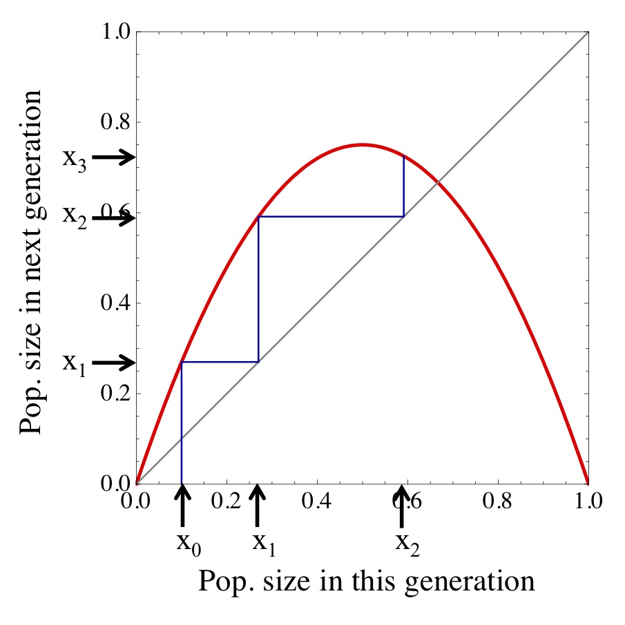Figure. 2: Illustration of the graphical method for understanding the dynamical behaviour of discrete-time models. See main text for explanation.

But how can we go beyond one time step in the future? Essentially, what we need to do is to use our old future time point (value along the y axis) as our new current time point. This can be achieved through an ingenious little trick: we can move horizontally to the main diagonal (i.e., the identify relation \(g(x)=x\)) and from there vertically again to our function \(f\), yielding the value of the variable at the next time point. Using again the logistic growth model as an example, this process is illustrated in Fig. (2).

2.6 Equilibria and their stability

The graphical method reveals that we can understand the dynamics of the model by moving back and forth between the function \(f\) defining the model and the main diagonal. But what happens when these two intersect?

The answer is that such intersections represent equilibria, or fixed points of the model, that is points where a variable does not change at all from one time point to the next. Identifying these equilibria and studying their properties is one of the most fundamental tasks for analysing any dynamical model. We can define an equilibrium point \(\widehat{x}\) as one where applying our model function doesn’t have any effect, i.e. where

\[\begin{equation} \tag{2.9} f(\widehat{x})=\widehat{x}. \end{equation}\] Thus, in our example of the logistic growth model, we can find the equilibria by solving the equation \[\begin{equation} \tag{2.10} b(1-\widehat{x})\widehat{x}=\widehat{x}. \end{equation}\]

for \(\widehat{x}\), yielding the two equilibria \(\widehat{x}_1=0\) and \(\widehat{x}_2=1-1/b\). The first equilibrium, \(\widehat{x}_1=0\), is sometimes referred to as the trivial fixed point. It simply means that when there are no individuals in the population, there never will be any since migration is not considered in the model. The second equilibrium is more interesting. You can see that this equilibrium takes positive values only when \(b>1\). This makes sense because as in the exponential model, the population is not sustainable when each individual produces less than one offspring individual on average. The greater \(b\) gets, the greater does the equilibrium become, reaching a maximum value of \(\widehat{x}_2=3/4\) when \(b=4\).

An important property of equilibria is their stability. An equilibrium is called locally stable if the system converges to the equilibrium when starting from sufficiently close by. Conversely, an equilibrium is called locally unstable if small perturbations away from the equilibrium result in the system moving entirely away from it. Fortunately, there is a simple recipe that allows one to determine whether an equilibrium is stable or unstable:

Obtain the derivative \(f'\) of the function \(f\) that defines the recursion equation.
Insert the formula for the equilibrium (e.g., \(f'(\widehat{x})\)) and simplify.
If the absolute value of this expression is less than one, the equilibrium is locally stable; if it is greater than one, the equilibrium is unstable. Moreover, if this expression is negative, there will be oscillations around this equilibrium.

Let’s use this recipe to determine the stability of the two equilibria in the logistic model. From Eq. , we can see that the function defining the recursion equation is \(f(x)=bx(1-x)\). For step one, we can use the product rule to calculate

\[\begin{equation} \tag{2.11} f'(x)=b(1-x) + bx(-1)=b(1-2x). \end{equation}\]

Inserting \(\widehat{x}_1=0\) gives simply \(f'(\widehat{x}_1)=b\). Applying the above criterion, we can see that the ‘trivial’ equilibrium \(\widehat{x}_1=0\) is stable if \(b<1\) but unstable if \(b>1\). This is in accord with our expectation. When \(b>1\), even a small initial population should lead to population growth so that we should move away from this equilibrium. Inserting the second equilibrium, \(\widehat{x}_2=1-1/b\) produces \(f'(\widehat{x}_2)=2-b\). The absolute value of this expression turns out to be less than one for \(1<b<3\), so that for those values of \(b\) the equilibrium is predicted to be stable. Moreover, \(f'(\widehat{x}_2)\) will be negative when \(b>2\) so that in this case we expect oscillations around the equilibrium.

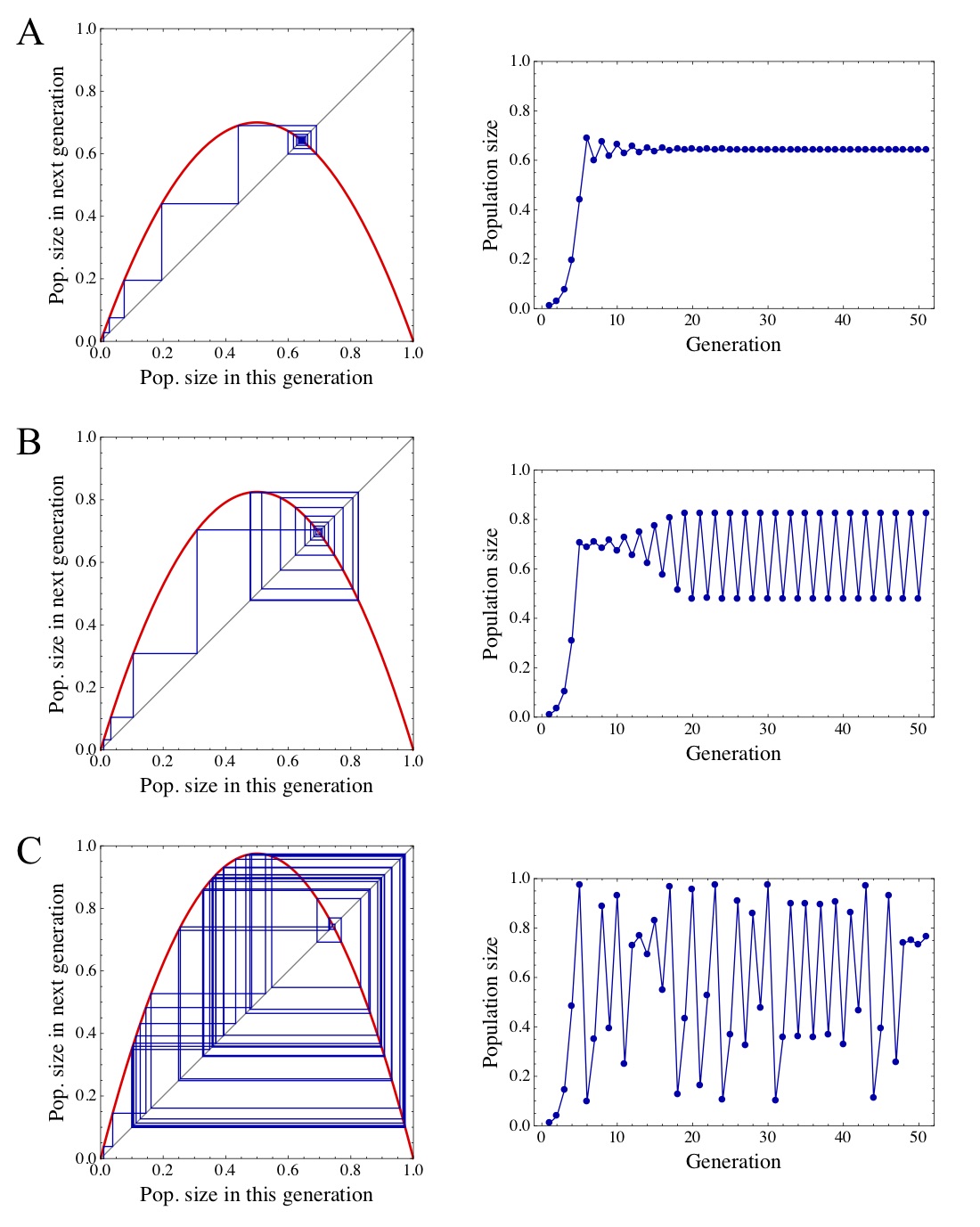Figure. 3: Three examples for possible dynamical behaviour of the logistic growth model. The plots on the left side illustrate the graphical method and the plots to the right show the population sizes against time. The parameter \(b\) takes values of (A) 2.8, (B) 3.3, and (C) 3.9, and the initial population size was \(x_0=0.01\) for all three panels.

The following app lets you explore how the dynamics of the logistic model and compare the graphical method to the direct plotting of population size through time:

library(shiny)

plotGraphical <- function(rate = 2, initialPop = 5, maxPop = 50, gens = 100) {
    xLog <- seq(0, 1, 0.01)
    yLog <- rate * xLog * (1 - xLog)

    par(mfrow = c(1, 2), mar = c(5, 5, 0, 0), oma = c(0, 0, 1, 1), mgp = c(2.5, 1, 0))
    plot(y = yLog, x = xLog, type = "l", col = "red", ylim = c(0, 1), 
         xlab = expression('x'[t]), ylab = expression('x'[t + 1]), cex.lab = 2)
    
    lines(x = seq(0, 1, 0.01), y = seq(0, 1, 0.01), type = "l")
    
    x0 <- initialPop/maxPop
    y0 <- rate * x0 * (1 - x0)
    
    lines(x = c(x0, x0), y = c(0, y0), type = "l", col = "blue")
    lines(x = c(x0, y0), y = c(y0, y0), type = "l", col = "blue")
    
    x <- y0
    y <- rate * x * (1 - x)
    
    count <- 1
    while (y != x & count < gens) {
            lines(x = c(x, x), y = c(x, y), type = "l", col = "blue")
            lines(x = c(x, y), y = c(y, y), type = "l", col = "blue")   
        
            x <- y  
            y <- rate * x * (1 - x)
            
            count <- count + 1
    }
    
    x <- seq(0, gens, 1)
    y <- rep(NA, length(x))
    y[1] <- initialPop/maxPop
    for(i in 2:length(y)){
        y[i] <- rate * y[i - 1] * (1 - y[i - 1])
    }

    plot(x = x, y = y,ylim = c(0, 1), xlim = c(0, gens), xlab = "Generations", 
        ylab = "Population Size", type = "l", col = "dark blue", cex.lab = 2)
}

app <- shinyApp(
    ui = fluidPage(
        titlePanel("Graphical Method"),
   
    sidebarLayout(
        sidebarPanel(      
            sliderInput("rate", "Growth Rate:",
                min = 0.9, max = 4.1,
                value = 3.2, step = 0.1),
                 
            sliderInput("initPop", "Initial Population Size:",
                min = 5, max = 45,
                value = 5, step = 1),
                 
            sliderInput("gens", "Generations:",
                min = 50, max = 500,
                value = 100, step = 50)
     
            ),
    
            mainPanel(
                plotOutput("plot")
            ),
    
            "left"
        )
    ),

    server = function(input, output) {
        output$plot <- renderPlot({
            plotGraphical(rate = input$rate, initialPop = input$initPop, gens = input$gens)
        })
    }
)

runApp(app)

As a final task, let us look at different outcomes of the model and see whether our predictions for the stability of equilibria hold. Fig. (3) shows the dynamics with three different values of \(b\) but the same initial population size. In Fig. (3)A, the system converges to the equilibrium - this was expected since \(b<3\) in this example. However, it can be seen that initially, there is some “overshooting”, i.e. the population size becomes greater than the equilibrium and then oscillates between smaller and greater values before converging. This happens because \(b>2\) in this example. Fig. (3)B shows an example where \(b>3\) and hence the equilibrium \(\widehat{x}_2\) is unstable. Instead of converging to the equilibrium, the system now converges to stable oscillations between two different values. In Fig. (3)C, something even more surprising happens for \(b=3.9\). The system does neither converge to a stable equilibrium nor exhibits regular oscillations, but instead behaves completely erratically. This seemingly random behaviour, termed chaos, is startling because the recursion itself is not only very simple but also completely deterministic.

An important lesson from the discrete-time logistic growth model is therefore that very simple models can produce very complex dynamics. This was discovered in the 1970s (May 1976) and created quite a stir. It also contributed to the development of chaos theory, i.e. the theory of how unpredictability arises in deterministic dynamical systems.

2.7 Natural selection in a clonal population

As a final example for a recursion equation, let us consider how selection operates in a simple, clonal population. Now we will assume that the size of the population, \(N\), is constant (a common assumption in evolutionary genetics). We further assume that there are two different genotypes in the population (or, more generally, two different types of individuals that faithfully pass on their type to their offspring). We can call the two types \(a\) and \(A\). Type \(a\) produced \(k\) offspring individuals per round of reproduction and type \(A\) produces \((1+s)k\) offspring individuals. The parameter \(s\) (\(s\geq -1\)) is called the selection coefficient and determines whether \(A\) individuals have fewer (\(s<0\)) or more(\(s>0\)) offspring than \(a\) individuals. To keep things simple, we assume that there is only a single round of reproduction following which the parental generation dies.

If, at generation 0, there are \(n_a\) and \(n_A\) individuals of the two types, after reproduction there will be

\[\begin{equation} \tag{2.12} n^\circ_a(t)=kn_a(t) \quad \text{and} \quad n^\circ_A(t)=(1+s)kn_A(t) \end{equation}\]

juvenile individuals in the population. (The prime indicates juveniles and time \(t\) is now indicated in brackets rather than as a subscript.) Since we assume that population size is constant, strong density regulation has to occur now so that the total number of adult individuals in generation 1 is again \(N\). This can be achieved by dividing by the total number of juveniles and then multiplying by \(N\):

\[\begin{align} n_a(t+1) & =\frac{N}{n^\circ_a(t)+n^\circ_A(t)} n^\circ_a(t) \\ n_A(t+1) & =\frac{N}{n^\circ_a(t)+n^\circ_A(t)} n^\circ_A(t) \tag{2.13} \end{align}\]

(Check that now the total population size always becomes \(N\)!) After inserting the formulae for \(n^\circ_a(t)\) and \(n^\circ_A(t)\) from Eq. (2.12) we get

\[\begin{align} n_a(t+1) & = \frac{N}{kn_a(t)+(1+s)kn_A(t)} kn_a(t) \\ n_A(t+1) & = \frac{N}{kn_a(t)+(1+s)kn_A(t)} k(1+s)n_A(t). \tag{2.14} \end{align}\]

After some simplification, this becomes

\[\begin{equation} \tag{2.15} n_a(t+1) = \frac{n_a(t)N}{n_a(t)+(1+s)n_A(t)} \end{equation}\] \[\begin{equation} \tag{2.16} n_A(t+1) = \frac{(1+s)n_A(t)N}{n_a(t)+(1+s)n_A(t)} \end{equation}\]

You can see that the parameter \(k\) has cancelled out and is therefore no longer part of the model! This means that the absolute number of offspring that an individual produces is irrelevant in the model - all that counts is the relative number of offspring, as determined by the selection coefficient \(s\).

Our model is now fully specified as a set of two recursion equations for two variables (\(n_a\) and \(n_A\)) and with parameters \(N\) and \(s\). In principle, we could therefore now start analysing it. However, before we do this we can try to simplify it further. This can be done by introducing a new variable, the frequency (or relative proportion) of individuals that are of type \(A\). This variable can be defined as

\[\begin{equation} \tag{2.17} p(t)=n_A(t)/N. \end{equation}\]

Equipped with this new variable, we can divide both sides of Eq. (2.16) by \(N\) to yield

\[\begin{equation} \tag{2.18} \frac{n_A(t+1)}{N} =p(t+1) = \frac{(1+s)n_A(t)}{n_a(t)+(1+s)n_A(t)}=\frac{(1+s)n_A(t)}{N+s n_A(t)} \end{equation}\]

(The last equality exploits the fact that \(n_a(t)+n_A(t)=N\).) As a final step, we can replace \(n_A\) by \(Np(t)\) (which follows from Eq. (2.17) to get

\[\begin{equation} \tag{2.19} p(t+1) =\frac{(1+s)Np(t)}{N+s Np(t)}=\frac{(1+s)p(t)}{1+s p(t)} \end{equation}\]

We have now arrived at a classic equation in population genetics. Our transformation has achieved two things. First, the parameter \(N\) has now also cancelled out, indicating that the total number of individuals also does not really matter for the model if we are only interested in the relative abundances (or frequencies) of the two types of individuals. Second, we have ended up with only a single, fully specified recursion equation for our model. This was possible because the frequency of type \(A\) and the frequency of type \(a\) must add up to one, so that it is sufficient to follow one of them in our model. As a result, our model (2.19) is now much simpler than the untransformed but mathematically equivalent model ((2.15) and (2.16)), consisting of only a single recursion equation instead of two and having only a single parameter instead of three.

We can now analyse the model in the same way as the population dynamics models in the previous sections. First, let’s find the equilibria of the model. We can note that if \(s=0\), then \(p(t+1)=p(t)\) will always be true: when there is no difference in the number of offspring produced by the two types, there will be no change. This is a rather boring case, so let’s exclude it from now on and assume that \(s\neq0\). We can then find the equilibria by solving

\[\begin{equation} \tag{2.20} \widehat{p} =\frac{(1+s)\widehat{p}}{1+s \widehat{p}} \end{equation}\]

for \(\widehat{p}\). One of the solutions, \(\widehat{p}_1=0\) is relatively easy to spot. Dividing both sides by \(\widehat{p}\) and rearranging then gives the only other equilibrium, \(\widehat{p}_2=1\). Thus, the system is at equilibrium if and only if type A is either extinct or ubiquitous (“fixed”) in the population.

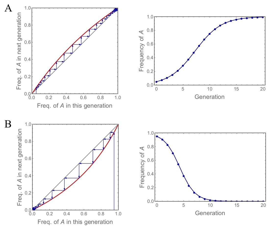Figure. 4: Two examples for possible dynamical behaviour of the natural selection model. The plots on the left side illustrate the graphical method and the plots to the right show the frequency of type \(A\) against time. The parameter \(s\) takes values of (A) 0.5 (selection for A) and (B) -0.5 (selection against A).

Second, we can determine the stability of these two equilibria by calculating the derivative of the function \(f(p)\) defining our recursion equation. Applying the quotient rule, this turns out to be

\[\begin{equation} \tag{2.21} f'(p)=\frac{(1+s) \times(1+sp)-(1+s)p \times s}{(1+s p)^2}=\frac{1+s}{(1+s p)^2} \end{equation}\]

Inserting our first equilibrium, \(\widehat{p}_1=0\) into this gives simply \(1+s\). Applying our criterion for stability, this demonstrates that \(\widehat{p}_1\) is stable if \(s<0\) and unstable if \(s>0\). This makes a lot of sense: if individuals with the \(A\) type produce fewer offspring than \(a\) individuals (which they do when \(s<0\)), they will always go extinct. Conversely, if \(A\) individuals produce more offspring than \(a\) individuals (\(s>0\)), introducing just a few \(A\) individuals will result in their spread within the population, i.e. their extinction is unstable.

Inserting our second equilibrium, \(\widehat{p}_2=1\) into Eq. (2.21) gives \(1/(1+s)\). Therefore, we have the opposite conditions for stability: \(s<0\) means fixation of type \(A\) is unstable, whereas \(s>0\) means fixation of \(A\) is stable.

Fig. (4) applies the graphical method to our model and shows two example dynamics for positive and negative selection on \(A\). The app below allows you to explore the dynamics of natural selection in an interactive manner.

library(shiny)

alleleFreq <- function(freqA = 0.5, s = 0.5, gen = 20) {
    generations     <- 0:gen
    frequency       <- rep(NA, length(generations))
    frequency[1]    <- freqA
        
    for (i in 1:gen) {
        frequency[i+1]  <- ((1 + s) * frequency[i])/(1 + s * frequency[i])
    }

    par(mar = c(5, 5, 0, 0), oma = c(0, 0, 1, 1), mgp = c(2.5, 1, 0))
    plot(NA, ylim = c(0, 1), xlim = c(0, gen), ylab = "Allele Frequencies", 
         xlab = "Generation", cex.lab = 2)
    polygon(x = c(0, gen, gen, 0), y = c(1, 1, 0, 0), col = "blue")
    polygon(x = c(gen, 0, 0:gen), y = c(0, 0, frequency), col = "red")
}

app <- shinyApp(
    ui = fluidPage(
        titlePanel("Allele Frequencies"),
   
        sidebarLayout(
            sidebarPanel(
                sliderInput("freqA", "Initial frequency of allele A:",
                            min = 0, max = 1,
                            value = 0.5, step = 0.1),
     
                sliderInput("s", "Selection coefficient:",
                            min = -1, max = 1,
                            value = 0.5, step = 0.1), 
                sliderInput("gen", "Number of generations:",
                            min = 10, max = 50,
                            value = 20) 
            ),
    
            mainPanel(
                plotOutput("plot")
            ),
        
            "right"
        )
    ),
      
    server = function(input, output) {
        output$plot <- renderPlot({
            alleleFreq(freqA = input$freqA, s = input$s, gen = input$gen)
        })
    }
)
    
runApp(app)

2.8 Exercises

1. The Ricker model (Ricker 1954) is a population dynamic model that is often used in fishery management. It can be expressed by the following recursion equation:

\[\begin{equation} N_{t+1}=N_t e^{r\left(1-\frac{N_t}{K}\right)} \end{equation}\]

Use the graphical method to gain some first insights into the behaviour of this model.
What are the equilibria of this model?
Determine the stability of the equilibria.
How does this model compare to the logistic model?

2. Our simple natural selection model assumed that there is only a single, closed population in which the dynamics take place. One extension of this model that relaxes this assumption might assume that there is continuous migration from another population consisting of only \(A\) type individuals. This model can be described by the recursion equation

\[\begin{equation} p_{t+1}=m+(1-m)\frac{(1+s)p_t}{1+sp_t}. \end{equation}\]

Provide an intuitive explanation for this equation and the new parameter \(m\).
What are the equilibria of this model?
Determine the stability of the equilibria.
Use the graphical method to gain additional insights into your model and compare the plot with your analytical results.
How does migration impact the dynamics compared to the simpler, one-population model?

3. The polymerase chain reaction (PCR) is a powerful and very widely used molecular method to amplify DNA fragments. You will probably have come across this method in other courses, but if you don’t remember how it works take a look at the excellent article on Wikipedia. For this exercise, develop a model for the number of DNA fragments after each round of amplification, making the following assumptions in different versions of your model:

Assume that there is always an excess of primers and nucleotides present in the solution, and that all DNA fragments are copied in each round of replication.
Assume that there is always an excess of primers and nucleotides present in the solution, but that now a certain fraction of DNA fragments fails to replicate in each round.
Assume that all DNA fragments can be replicated in principle but that now primers are no longer present in excess. (There might be enough primers for the first few rounds but not for later rounds.) Nucleotides are still always present in excess.
Finally, assume that all DNA fragments can be replicated in principle and that primers are always present in excess, but that the amount of free nucleotides in the solution can become limiting. To keep the model simple, just assume that a certain fixed number of nucleotides is required toreplicating one DNA molecule, but don’t distinguish between different types of nucleotides. Note that this model version is more challenging than the others in that it will probably require more than one variable!

References

May, R.M. 1976. “Simple Mathematical Models with Very Complicated Dynamics.” Journal Article. Nature 261: 459–67.

Ricker, W. E. 1954. “Stock and Recruitment.” Journal Article. Journal of the Fisheries Research Board of Canada 11 (5): 559–623.