Lecture 5 A glimpse into stochastic models

To conclude this course we will take a look at stochastic models, i.e. models in which the variables change randomly. Such models are more difficult to analyse mathematically. It’s also more difficult to simulate them on a computer because it is now necessary to run the model not only once but many times and then study the resulting distribution of outcomes. At the same time, most biological process are intrinsically stochastic, so that stochastic models are usually more realistic than deterministic ones. This, and the rapid pace at which computer power has increased in the last decades, has made stochastic models increasingly popular. Stochastic models are now the state-of-the-art in ecology (e.g., neutral models of biodiversity), population genetics (e.g., the coalescent process), and evolution (e.g., methods to estimate phylogenetic trees). Here, we will try to obtain a first, broad understanding of important classes of stochastic models (mathematically: stochastic processes), again with examples from ecology and evolution. Table provides an overview of the stochastic processes that we will cover. All these processes of models can be regarded as special cases of a larger class of stochastic processes called Markov processes. Markov processes are characterised by being “memoryless”, which means the change in variables is influenced only by their present but not by their past states. For a more in-depth, but still (relatively) accessible treatment of stochastic processes in biology, see Ref. (Allen 2003).

Stochastic process	Time	Characteristics	Examples
Branching process	discrete or continuous	population model where each individual’s offspring number is drawn from same distribution	colonization of new habitat, spread of new disease
Markov chain	discrete	switches between different states, with probabilities depending on previous state	nucleotide substitutions in DNA sequence evolution
Poisson process	continuous	events that happen independently and with a small probability per unit of time	mutations in lineage of individuals, coalescent process
Wiener process	continuous	random changes in variable but with mean zero	movement of individuals in space

5.1 Branching processes

Branching processes can be understood as population models in which offspring numbers are independent and identically distributed random variables. For examples, let us assume a population in which each individual \(i\) produces \(k_i\) offspring, with \(k_i\) ranging from 0 to 2. All \(k_i\) are distributed according to the following distribution:

\[\begin{equation} \tag{5.1} k_i=\begin{cases} 0 & \text{with probability } p_0=0.2 \\ 1 & \text{with probability } p_1=0.5 \\ 2 & \text{with probability } p_2=0.3 \\ \end{cases} \end{equation}\]

Denoting population size at time \(t\) by \(N_t\) and assuming that all adult individuals die after reproduction (the same ‘discrete generations’ assumption we made in recursion equation models in Lecture 2), we can then write down the model as

\[\begin{equation} \tag{5.2} N_{t+1}=\begin{cases} 0 & \text{if } N_t=0 \\ \sum_{i=1}^{N_t} k_i & \text{if } N_t>0 \\ \end{cases} \end{equation}\]

Figure (1) shows an example for the population dynamics of this model. It is not difficult to work out from the probabilities in Eq. (5.1) that the expected number of offspring is 1.1 for all individuals (\(E[k_i]=0\times 0.2 + 1 \times 0.5 + 2 \times 0.3 =1.1\)). Therefore, on average, we would expect the population to be able to grow. However, as this is a stochastic model, extinction is possible nonetheless and an important question in branching process is with what probability extinction occurs. This and other questions can be addressed very elegantly using probability generating functions, but we will not pursue this here.

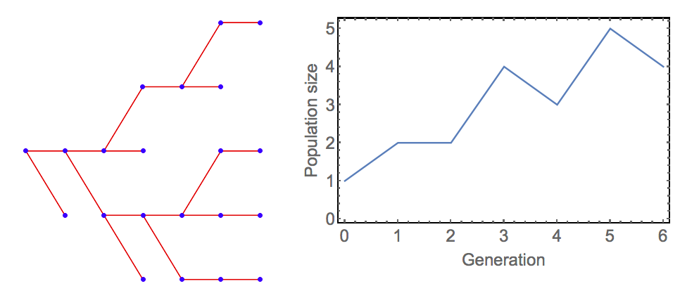Figure. 1: Example dynamics of the branching process model specified in Equations (5.1) and (5.2). The left panel shows the genealogy of the population (the ‘branching’) and the left panel shows population size through time. (Figure produced using modified Mathematica code by Heikki Ruskeepää from Wolfram Demonstrations Project^TM ‘Simulating the Branching Process’

5.2 Markov chains

Branching processes are a special case of a class of discrete-time stochastic processes called Markov chains. In a Markov chain, a variable can take a number of discrete values that are called ‘states’. In each time step, those states can change to other states with certain probabilities.

As an example, consider the dynamics of nucleotide substitutions at a given site in the DNA of a species. The four states are the four nucleotides, i.e. the variable of our model can take any of the four values A, C, T and G. Through mutation and drift, this nucleotide can be replaced by a different nucleotide within a certain time period. In principle, one could assign each of the twelve possible substitutions (A\(\rightarrow\)C, A\(\rightarrow\)G, A\(\rightarrow\)T, C\(\rightarrow\)A, C\(\rightarrow\)G etc.) its own probability. Usually, however, simpler models with fewer parameters are used, and one of simplest is a classic two-parameter model by Kimura (Kimura 1980). The transition probabilities in this model are shown in Figure (2). Analysing this model is beyond the scope of this course but there are some results that are quite intuitive. For example, there is no absorbing state in this model, i.e. no state at which the system ‘gets stuck’ and doesn’t change anymore. Moreover, the model is completely symmetrical: even though in the beginning we might remain at the original nucleotide for some time, in the long run, all four states have the same chance of being reached. In other words, the equilibrium probability distribution of the four states is the vector \((\frac{1}{4},\frac{1}{4}, \frac{1}{4}, \frac{1}{4})\) in this model.

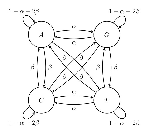Figure. 2: Kimura’s model for nucleotide substitutions. Transition substitutions between different purins or pyrimidins (A <-> G or C <-> T) occur with probability \(\alpha\) whereas transversions (from purine to pyrimidine or vice versa) occur with a lower probability \(\beta\). Thus, in total the probability that a base changes in one time step is \(\alpha+2\beta\) and the probability that it does not change is \(1-\alpha-2\beta\).

As a second example, consider a (grossly unrealistic) model of species extinction in which a species can have three different conservation statuses: ‘no concern’ (N), ‘threatened’ (T) and ‘extinct’ (E). Assuming that within one timestep a species can only change from one of these categories to an adjacent one this model could be parameterised as:

Figure. 3: A simple model of species extinction. Species can exist in one of three states: ‘no concern’ (N), ‘threatened’ (T) and ‘extinct’ (E). Species can pass from N to T at a rate determined by \(\alpha\), and from T to N at a rate determined by \(\beta\). Once species pass from T to E (at a rate of \(\gamma\)), they will remain in this state permanently.

In this model, we now do have an absorbing state, the state \(E\). Sadly, when \(\alpha>0\) and \(\gamma>0\) state \(E\) will eventually be reached and then maintained indefinitely.

Markov chains and their various extensions and applications play a central role in computational biology. One important extension are Hidden Markov Models. Here, the states of the process are hidden, i.e. they cannot be observed. Instead, there are other, observable states that are generated (“emitted”) with certain probabilities by the hidden states. Predicting the sequence of hidden states, the transition and the emission probabilities given a sequence of observed states is very challenging, but clever algorithms have been developed that rise to the challenge. Hidden Markov Models are widely used in bioinformatics, for example in methods of predicting protein folding, DNA sequence alignment and gene prediction.

An important application of Markov chains are Markov Chain Monte Carlo (MCMC) methods. There are many problems in biology where one would like to estimate complex probability distributions. One example arising in the field of phylogenetics is the distribution of probabilities of different phylogenetic trees explaining the evolutionary relationship between species, given certain DNA sequence data for the species. Within a Bayesian framework, one can estimate the probability of a tree given the data (the posterior probability) from the probability of observing these data given the tree (the likelihood of the tree). This is achieved through various models of DNA sequence evolution. Unfortunately, because the number of possible trees is usually ginormous, it is impossible to calculate this probability for all trees. Here is where MCMC comes in: instead of trying to go through all trees (impossible) or selecting a random set of trees (very inefficient), a kind of random walk through the forest of trees is performed. Starting with a randomly chosen tree, it’s likelihood is estimated. Then, another tree that is similar to the first one is randomly chosen and it’s likelihood is also determined. Depending on these two likelihoods and the exact algorithm that is used (a popular choice is the Metropolis-Hastings algorithm), one either proceeds to the new tree or stays with the old tree. This process is repeated many times. The beauty of MCMC is that the relative number of time steps that the process spends in the different states (here: trees) will converge to the underlying probability distribution of these states. In other words, MCMC allows one to obtain samples from a complex probability distribution.

5.3 Poisson processes

Poisson processes are processes in which certain events happen independently from each other and with a small, constant probability per unit of time. For example, these events could be customers arriving in a shop, radioactive particles decaying or shooting stars. Poisson processes have been studied for a long time and have a number of simple properties that make them attractive. Most importantly, the number of events that occur within any given time interval follows a Poisson distribution (hence the name Poisson process). Moreover, the time interval between two successive events follows an exponential distribution. Figure (4) shows an instance of a Poisson process illustrating these expectations. Poisson processes could also include several different types of events that occur with different probabilities.

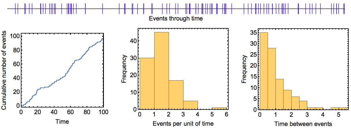Figure. 4: Example run of a Poisson process. In this process, events occured at a rate of \(\lambda=1\) per unit of time and the process was run over 100 time units. The upper panel shows events (blue bars) as they occurred through time. The plots in the lower panel show the cumulative number of events that had occurred at different time points, the distribution of the number of events during the 100 time intervals of length one, and the distribution of times between consecutive events. The theoretical expectation for these three quantities is a line with slope \(\lambda\), a Poisson distribution with mean (and variance) \(\lambda\), and an exponential distribution with mean \(1/\lambda\), respectively.

In theoretical ecology and evolutionary biology, Poisson processes have a central role. For example, when considering an evolving species through time, the accumulation of mutations in this species can be modelled as a Poisson process. This could then be the basis for statistical methods to estimate the rate at which mutations accumulate, or for methods to estimate the time at which an ancestral species split into two extant species. Poisson processes can also be part of more complex stochastic processes such as the coalescent, an important model in modern population genetics (see (Wakeley 2009) for an introduction).

5.4 Wiener processes

Wiener processes – also called Brownian motion processes – are continuous-time processes in which one or several variables are subject to small random fluctuations. More precisely, the changes in the variable(s) in infinitesimally small time steps follow a normal distribution with mean zero and a constant variance that determines the speed of the process. Any changes in the variable(s) are independent of previous changes (the Markov or ‘memorylessness’ property). The result is a kind of random walk where both time and space are continuous. The process is illustrated in Figure (5) for both one and two variables (or spatial dimensions).

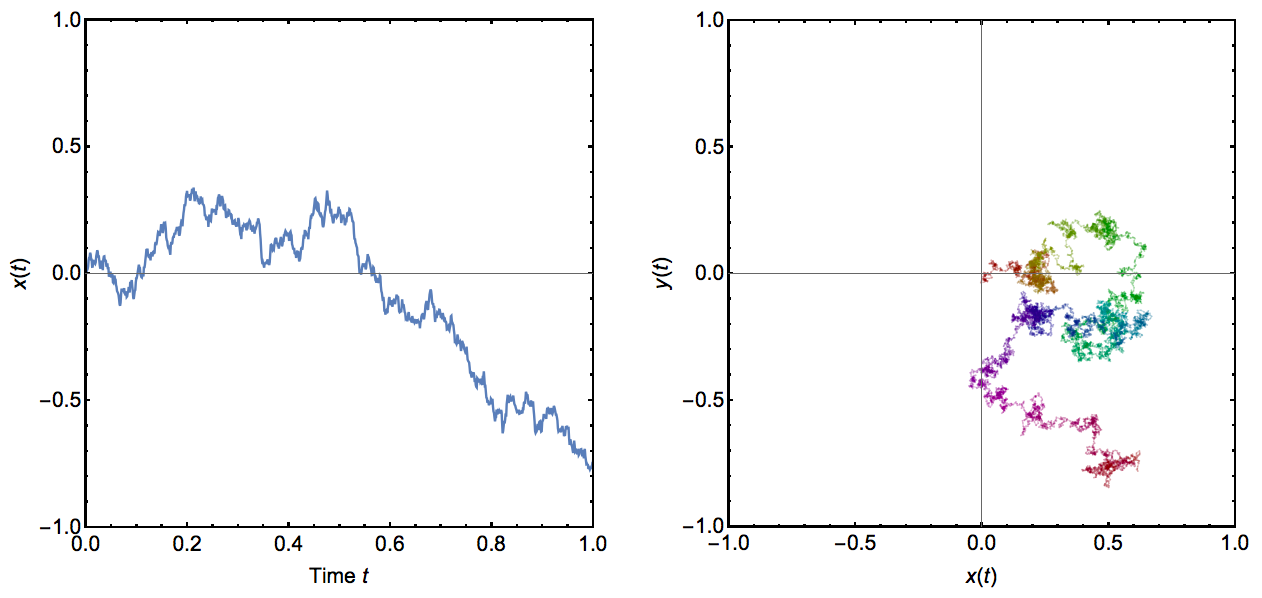Figure. 5: Example runs of Wiener processes. In the left panel, a Wiener process with a single variable is shown through time. The right panel shows a Wiener process in two variables, which could be interpreted for example as a random walk in two dimensions. Time is indicated here by color, changing from red at time \(t=0\) via yellow, green, blue and purple to red again at time \(t=1\). In all cases, the variance parameter for this process was set to 0.5.

Wiener processes can be used for example as null models for the movement of organisms in space. Such a movement could be described as a kind of ‘aimless wandering around’, in contrast perhaps to a more systematic exploration of the habitat or a directed movement towards some goal. Wiener processes have also been used extensively to model how continuous traits change through time in a clade of evolving species.

5.5 Concluding remarks

The take-home message from this lecture is that there are many stochastic processes that are well-studied and that can be used to model biological phenomena. We have not studied these processes in any mathematical detail and we have barely scratched the surface of what’s out there. However, you should now be aware of what kind of models exist and that they have been extensively studied by mathematicians. Therefore, if you encounter a problem that a stochastic model might shed light on, don’t reinvent the wheel and start writing a simulation program immediately. Instead, check whether your problem might be covered by one of the many stochastic processes that clever mathematicians have discovered. If so, deep mathematical results on the behaviour of the model might readily be available, potentially rendering any simulations superfluous.

One aspect that we haven’t been able to discuss much here is the connection between stochastic models and data. This is where the two quantitative modules of this course (statistical and mathematical modelling) would naturally merge. For example, one common application of stochastic models is to infer the parameters of the model with empirical data. This can be done for example by estimating the probability of observing the data for a given set of model parameters. This is called the likelihood of the parameters, and its maximum across all possible parameter values is the maximum likelihood (ML) estimate of those parameters. ML as well as Bayesian approaches can also be used to assess how well competing stochastic models explain the data.

5.6 Exercises

1. Consider the following phenomena:

1. A small uninhabited island experiences volcanic eruptions. These eruptions occur with a small probability in each year and obliterate all vegetation. Upon such an event, there is a small yearly probability that the island might get re-colonised by early pioneer species (e.g., lichens). Next, those species will be succeeded by herbaceous plants and eventually by a stage where shrubs and trees grow.
2. Microsatellites are DNA sequences where short DNA motives are repeated many (~5 to 50) times. They arise by DNA strand slippage during replication that can either reduce or increase the number of repeats. In this way, microsatellites can grow or shrink in length, and the resulting polymorphisms that arise within natural populations have been widely used as markers in population genetics, forensics and paternity testing.
3. A plant population reproduces exclusively by selfing (ovules fertilised by pollen from the same plant). Initially, a certain number of loci are observed to be heterozygous but in each generation there is a probability of \(1/2\) that any given locus will become homozygous. Assuming no selection, mutation or any other evolutionary forces, one might be interested to know what the expected time is until a certain lineage has become fully homozygous.

For each phenomenon, determine what kind of stochastic process might be suitable to model it. Explain, specify the model and draw a diagram to illustrate it.

2. As briefly mentioned, branching processes are a special type of a Markov chain. Explain why this is the case and formulate the example model of stochastic population growth (section 5.1 as a Markov chain. How is this Markov chain different from the ones we considered in section 5.2?

References

Allen, L. J. S. 2003. An Introduction to Stochastic Processes with Applications to Biology. Book. Upper Saddle River, N.J.: Pearson/Prentice Hall.

Kimura, M. 1980. “A Simple Method for Estimating Evolutionary Rates of Base Substitutions Through Comparative Studies of Nucleotide-Sequences.” Journal Article. Journal of Molecular Evolution 16 (2): 111–20. doi:Doi 10.1007/Bf01731581.

Wakeley, J. 2009. Coalescent Theory: An Introduction. Book. Greenwood Village, CO, USA: Roberts; Company Publishers.