Lecture 3 Continuous-time models in one variable

Continuous-time models generally take the shape of differential equations. Since this is a fairly advanced topic in mathematics usually not taught below university level, we will start with a very short introduction to differential equations. We will then look at some examples of continuous time models of population growth, mirroring the discrete-time examples covered in the previous section. Finally, as the most important properties of dynamical models, we will again look at equilibria and their stability in continuous-time models.

3.1 What are differential equations?

Equations that you should be familiar with are something like

\[\begin{equation} \tag{3.1} x+x^2=6. \end{equation}\]

After some pondering and unearthing cheerful memories from high school maths, you may find that the solutions to this equation are \(x=2\) and \(x=-3\). In equations like this, we are looking for numbers that, when inserted for a variable (in this case \(x\)), turn the equation into a true statement. There may be one solution, several solutions (as in the example), infinitely many solutions or no solution at all.

Differential equations are equations in which the unknown object is not a number, but a function. Moreover, these equations involve not only the function, but also derivatives of that function. Consider the following example:

\[\begin{equation} \tag{3.2} y(t)(1-2t)=ty'(t) \end{equation}\]

In this differential equation, we want to solve for \(y\), which is an unknown function of the variable \(t\). The equation involves the function \(y(t)\) itself, its first derivative \(y'(t)\), and the variable \(t\). Finding the solution to differential equations can be very tricky, but this does not need to concern us in this course. On the other hand, once you’ve come up with a possible solution, it is fairly easy to verify that this is indeed a solution. A solution of the above differential equation is

\[\begin{equation} \tag{3.3} y(t)=te^{-2t} \end{equation}\]

To show that this is a solution, we can first use the product rule of calculus to obtain the derivative of \(y(t)\),

\[\begin{equation} \tag{3.4} y'(t)=(1-2t)e^{-2t}. \end{equation}\]

Plugging both \(y(t)\) and \(y'(t)\) into Eq. (3.2) and simplifying the result then confirms that (3.3) is indeed a solution to (3.2). To complete this example, one can also readily show (try it!) that any function

\[\begin{equation} \tag{3.5} y(t)=Cte^{-2t}, \end{equation}\]

where \(C\) is an arbitrary real number, is a solution to to Eq. (3.2). This means that there are infinitely many solutions \(y(t)\) that satisfy our example differential equation.

Finally, we need some basic terminology to classify different types of differential equations. Eq. (3.2), and in fact every differential equation we will be dealing with here, is an ordinary differential equation, or short ODE. This simply means that the unknown function is a function of only a single variable (\(t\)). Differential equations in more than one variable are called partial differential equations and are much more difficult to deal with. Eq. (3.2) is said to be of first order, meaning that only the first derivative shows up. Finally, Eq. (3.2) is a linear differential equation because it represents a linear relationship between \(y(t)\) and its derivatives. (In other words, no non-linear terms such as \(y(t)^2\) or \(\cos(y(t))\) occur.) We will deal with both linear and non-linear ODEs.

3.2 An ODE model of exponential population growth

The first discrete-time model for population growth was one where we assumed that in each time step, every individual produces a certain, fixed number of offspring. So, let’s try to do the same with continuous time and using an ODE! What this means is that we will now assume that individuals in the population reproduce continuously throughout the year. Informally, we can arrive at the ODE by assuming that there is a constant rate at which new offspring are produced per parent individual and per unit of time. In other words, the rate at which the population grows (or the “slope” of population increase) is proportional to the number of individuals already present:

\[\begin{equation} \tag{3.6} N'(t)=rN(t), \end{equation}\]

In this ODE, \(N\) is the function we are looking for, and \(t\) is the independent variable of that function. The ODE is linear and of first order.

We can also derive this differential equation more formally by starting from the corresponding discrete time model \(N_{t+1}=a N_t\) (Section 2.3). Rewriting this model, we have

\[\begin{equation} \tag{3.7} \Delta N=N_{t+1}-N_t=(a-1)N_t, \end{equation}\]

which is called a difference equation. This can also be written as

\[\begin{equation} \tag{3.8} N(t)-N(t+\Delta t)=(a-1)\Delta t N(t). \end{equation}\]

In the discrete-time model, \(\Delta t=1\), but now we would like to reduce the step size \(\Delta t\) to an infinitesimally small value. Dividing both sides by \(\Delta t\) yields

\[\begin{equation} \tag{3.9} \frac{N(t)-N(t+\Delta t)}{\Delta t}=\frac{(a-1)\Delta tN(t)}{\Delta t}=(a-1)N(t). \end{equation}\]

Now, if we let \(\Delta t\) go to zero, the left hand side of the equation converges to the derivative of \(N\) with respect to \(t\), so that we arrive at the differential equation

\[\begin{equation} \tag{3.10} \lim_{\Delta t\rightarrow 0}\frac{N(t)-N(t+\Delta t)}{\Delta t}=\frac{dN(t)}{dt}=N'(t)=rN(t), \end{equation}\]

with \(r\) defined as \(r:=a-1\).

Now that we have specified our model (the ODE in Eq. (3.6)), how do we go about analysing it? In this simple case, we can find an actual solution of the model:

\[\begin{equation} \tag{3.11} N(t)=N_0e^{rt} \end{equation}\]

To confirm that this is indeed a solution of the ODE for all possible values of \(N_0\), we can calculate the derivative of the solution as \(N'(t)=rN_0e^{rt}\). This demonstrates that indeed, as required by our ODE, \(N'(t)=r(N_0e^{rt})=rN(t)\).

The solution of the ODE gives us everything we need to understand how the model will behave. When \(t=0\), \(N(t)=N_0\). So, the population size takes its initial value, the aptly named \(N_0\). When \(N_0=0\) (no individuals to start with), the population size remains at zero no matter how large the growth rate is, which makes a lot of sense. When \(N_0>0\), \(N\) increases exponentially through time when \(r>0\), i.e. for positive growth rates. For negative growth rates \(r<0\) (which effectively are death rates), the population shrinks exponentially towards zero. When \(r=0\) the population sizes remains constant through time.

For most ODEs, no solution can be found. This is not because mathematicians haven’t been clever enough to find a solution - they have proven that for many ODEs a solution (technically: a “closed-form expression” of a solution) simply cannot be written down. In such cases, we need to rely on other techniques to extract information about the model. The most important of those techniques are again finding the equilibria of the model and determining their stability, which we will turn to next.

3.3 Equilibria and their stability in ODE models

In discrete-time models, we defined an equilibrium were no change occurred, e.g. where \(N_{t+1}=N_t\). The same definition applies to ODEs. However, now “no change” means no change in our continuous-time variables, which translates to \(N'(t)=0\). (Remember that the derivative of a function can be interpreted as how fast and in what direction the function value changes.) To find the equilibria of an ODE model, we can therefore set the right-hand side of the equation defining the ODE to zero and solve for the variable of interest. More formally, if the differential equation is of the form

\[\begin{equation} \tag{3.12} x'(t)=f(x(t)), \end{equation}\]

then we can find the equilibria by solving

\[\begin{equation} \tag{3.13} f(\widehat{x})=0 \end{equation}\]

for \(\widehat{x}\). In order to determine the stability of the equilibria, we can again follow a simple recipe:

1. Obtain the derivative \(f'\) of the function \(f\) that defines the ODE.
2. Insert the formula for the equilibrium (e.g., \(f'(\widehat{x})\)) and simplify.
3. If this expression is negative, the equilibrium is locally stable; if it is positive, the equilibrium is unstable.

Compare this recipe to the one we encountered for discrete-time models: the two are very similar but the final criterion is different. An intuition for this criterion can be gained by using again a graphical method that plots the function \(f\) defining the ODE. Consider for example the ODE model specified by the function \(f\) shown in Fig. (1). The function \(f\) is characterised by three intersections with the x-axis, corresponding to the three equilibria \(\widehat{x}_1\), \(\widehat{x}_2\) and \(\widehat{x}_3\). For values of \(x\) that are slightly less than \(\widehat{x}_1\), \(f\) takes negative values, whereas for values of \(x\) slightly greater than \(\widehat{x}_1\), \(f\) takes positive values. This situation is reflected in the fact that \(f'(\widehat{x}_1)>0\). What it means is that small perturbations of \(\widehat{x}_1\) to either side will result in \(x(t)\) moving away from this equilibrium over time, i.e. \(\widehat{x}_1\) is an unstable equilibrium. Conversely, since \(f'(\widehat{x}_2)<0\), small perturbations of \(x\) at \(\widehat{x}_2\) to either side will result in \(x(t)\) moving back to \(\widehat{x}_2\) over time. \(\widehat{x}_3\) is again an unstable equilibrium.

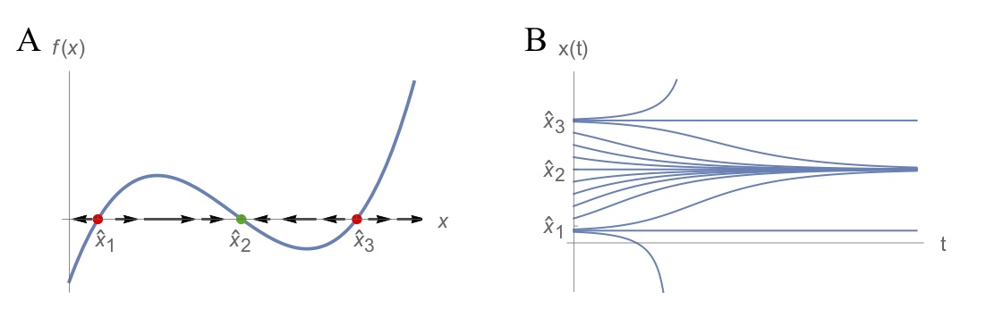Figure. 1: Illustration of the graphical method for understanding the dynamical behaviour of continuous-time models. The model is characterised by three equilibria of which \(\widehat{x}_1\) and \(\widehat{x}_3\) are unstable and \(\widehat{x}_2\) is stable. See main text for explanation.

3.4 Continuous-time logistic growth

In the previous lecture we’ve encountered the logistic recursion equation and saw that it can lead to very complex dynamics. There is also a continuous-time version of this model, given by the following ODE:

\[\begin{equation} \tag{3.14} N'(t)=rN(t)\left(1-\frac{N(t)}{K}\right) \end{equation}\]

You can see that this equation looks very similar to the logistic recursion equation \(N_{t+1}=b\left(1-\frac{N_t}{M}\right) N_t\) found in section 2.4. However, there are important differences in interpretation of the parameters. In the logistic recursion equation, \(b\) is the number of offspring produced by each individual in a small population, whereas here, \(r\) is the growth rate of the population per unit of time when the population size is small. Moreover, in the recursion equation \(M\) is the maximum possible population size (at which the population crashes) whereas \(K\) is the carrying capacity of the population, i.e. the population size where net growth is zero.

In order to identify the equilibria of the ODE in Eq. (3.14), we need to find values of \(N\) where the function \(f\) defining the ODE is zero:

\[\begin{equation} \tag{3.15} f(\widehat{N})=r\widehat{N}\left(1-\frac{\widehat{N}}{K}\right)=0. \end{equation}\]

Solving this equation for \(\widehat{N}\) yields the two equilibria \(\widehat{N}_1=0\) and \(\widehat{N}_2=K\). To find out under what conditions these equilibria are stable or unstable, let’s compute the derivative of \(f\):

\[\begin{equation} \tag{3.16} f'(N)=r \times \left(1-\frac{N}{K}\right) + rN \times \left(-\frac{1}{K}\right) =r \left(1-\frac{2N}{K}\right) \end{equation}\]

Plugging the expression for our two equilibria into this formula gives \(f'(\widehat{N}_1)=r\) and \(f'(\widehat{N}_2)=-r\). Applying the recipe for stability in ODEs, this means that provided \(r>0\) (positive growth in the absence of any competition), the equilibrium \(\widehat{N}_1=0\) is always unstable whereas the equilibrium \(\widehat{N}_2=K\) is always stable. Note that this is in marked contrast to the complex dynamics we’ve encountered in the discrete time version of the model. Although ODEs can also exhibit complex dynamics (cycling, chaos) they do so less readily than recursion equations. In particular, when there is only a single variable, chaotic behaviour never emerges in continuous time dynamical systems.

3.5 Exercises

1. Determine the equilibria and their stability for the exponential growth model in Eq. (3.6). Apply the graphical method to this model and compare your results with expectations from the solution of this model, as given in Eq. (3.11).

2. Demonstrate that the function

\[\begin{equation} N(t)=N_0 \frac{K e^{r t}}{K+N_0(e^{r t}-1)} \end{equation}\]

is a solution of the logistic ODE in Eq. (3.14), and verify that this solution is in accord with the equilibria and their stability, as derived above.

3. Harvesting prevents the population size of a species from attaining its natural carrying capacity. We can add harvesting to the logistic model by assuming that the per capita harvest rate is \(m\) per day in a population whose intrinsic growth rate is \(r\) per day and whose carrying capacity is \(K\) in the absence of harvesting.

1. Derive a differential equation describing the dynamics of the population.
2. Determine the equilibria for this model.
3. Determine the stability of these equilibria.
4. What conditions must hold for the population to persist?
5. What is the maximum allowable harvest rate that ensures that the population size will remain stable at a size greater than 1000?

(This is Problem 5.9 taken from (Otto and Day 2007).)

References

Otto, S. P., and T. Day. 2007. A Biologist’s Guide to Mathematical Modeling in Ecology and Evolution. Book. Princeton: Princeton University Press. http://www.loc.gov/catdir/enhancements/fy0704/2006044774-b.html.