10 Nonlinear Principal Component Analysis and princals()

10.1 Introduction

princals, principals, Shepard-Kruskal, mdrace, history

10.2 Equations

Suppose all \(m\) blocks each contain only a single variable. Then the Burt matrix is the correlation matrix of the \(H_j\), which are all \(n\times 1\) matrices in this case. It follows that MVAOS maximizes the sum of the \(r\) largest eigenvalues of the correlation matrix over transformations, i.e. MVAOS is nonlinear principal component analysis (De Leeuw 2014).

10.3 Examples

10.3.1 Thirteen Personality Scales

We use the same data as before for an NLPCA with all blocks of rank one, all variables ordinal, and splines of degree 2.

epi_copies <- rep (1, 13)
epi_ordinal <- rep (TRUE, 13)
h <- princals(epi, epi_knots, epi_degrees, epi_ordinal, epi_copies)

In 19 iterations we find minimum loss 0.7330409. The object scores are in figure 17 and the transformation plots in figure 18. NLPCA maximizes the sum of the two largest eigenvalues of the correlation matrix of the variables. Before transformation the eigenvalues are 4.0043587, 2.6702003, 1.9970912, 0.8813983, 0.6571463, 0.6299946, 0.5246896, 0.4657022, 0.3457515, 0.3403361, 0.2767531, 0.1835449, 0.0230333, after transformation they are 4.195697, 2.7452519, 1.603667, 0.8209126, 0.71826, 0.6769619, 0.5185328, 0.4544125, 0.419768, 0.3519542, 0.2932654, 0.170027, 0.0312897. The sum of the first two goes from 6.674559 to 6.9409489.

---

plot(h$objectscores, xlab = "dim1", ylab = "dim2", col = "RED", cex = .5)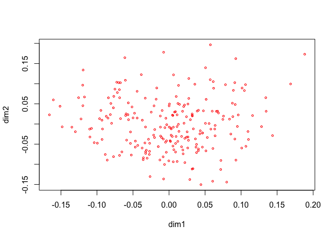

Figure 17: Personality Scales, Object Scores, Single Ordinal, Degree Two

---

---

Figure 18: Personality Scales, Transformations, Single Ordinal, Degree Two

---

We repeat the analysis with ordinal variables of degree two, without interior knots. Thus we the transformation plots will be quadratic polynomials that are monotone over the range of the data.

h <- princals(epi, knotsE(epi), epi_degrees, epi_ordinal)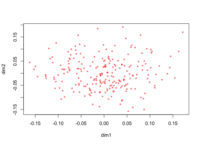

In 21 iterations we find minimum loss 0.7392792. The object scores are in figure 19 and the transformation plots in figure 20. The eigenvalues are now 4.0845453, 2.6942028, 1.8268476, 0.8731782, 0.6698534, 0.6503449, 0.540624, 0.4597014, 0.3666353, 0.3470226, 0.2847375, 0.1783405, 0.0239667, with sum of the first two equal to 6.778748.

---

Figure 19: Personality Scales, Object Scores, Single Numerical, Degree Two

---

---

Figure 20: Personality Scales, Transformations, Single Numerical, Degree Two

---

References

De Leeuw, J. 2014. “History of Nonlinear Principal Component Analysis.” In The Visualization and Verbalization of Data, edited by J. Blasius and M. Greenacre. Chapman; Hall. http://www.stat.ucla.edu/~deleeuw/janspubs/2014/chapters/deleeuw_C_14.pdf.