7 Multiple Correspondence Analysis and homals()
7.1 Introduction
Suppose all basis matrices \(G_{j\ell}\) in block \(j\) are the same, say equal to \(G_j\). Then the block scores \(H_jA_j\) are equal to \(G_jZ_jA_j\), which we can write simply as \(G_jY_j\). Thus loss must be minimized over \(X\) and the \(Y_j\).
If all \(G_j\) are binary indicators of categorical variables, and the \(m\) blocks are all of span one, then MVAOS is multiple correspondence analysis (MCA). The block scores \(G_jY_j\) are \(k_j\) different points in \(\mathbb{R}^p\), with \(k_j\) the number of categories of the variable, which is usually much less than \(n\). The plot connecting the block scores to the object scores is called the star plot of the variable. If \(k_j\) is much smaller than \(n\) a star plot will connect all object scores to their category centroids, and the plot for a block (i.e. a variable) will show \(k_j\) stars. Since loss \(\sigma\) is equal to the sum of squared distances between object scores and block scores, we quantify or transform variables so that stars are small.
In our MVAOS MCA function homals() we allow for B-spline bases and for monotonicity restrictions. The input data (as for all MVAOS programs) needs to be numeric, and we included a small utility function makeNumeric() that can be used on data frames, factors, and character variables to turn them into numeric matrices. All other arguments to the function have default values.
homals <-
  function (data,
            knots = knotsD (data),
            degrees = rep (-1, ncol (data)),
            ordinal = rep (FALSE, ncol (data)),
            ndim = 2,
            ties = "s",
            missing = "m",
            names = colnames (data, do.NULL = FALSE),
            itmax = 1000,
            eps = 1e-6,
            seed = 123,
            verbose = FALSE)
The output is a structure of class homals, i.e. a list with a class attributehomals. The list consists of transformed variables (in xhat), their correlation (in rhat), the objectscores (in objectscores), the blockscores (in blockscores, which is itself a list of length number of variables), the discrimination matrices (in dmeasures, a list of length number of variables), their average (in lambda), the weights (in a), the number of iterations (in ntel), and the loss function value (in f).
    return (structure (
      list (
        transform = v,
        rhat = corList (v),
        objectscores = h$x,
        scores = y,
        quantifications = z,
        dmeasures = d,
        lambda = dsum / ncol (data),
        weights = a,
        loadings = o,
        ntel = h$ntel,
        f = h$f
      ),
      class = "homals"
    ))
Note that in MCA we have \(H_jA_j=G_jY_j\). In previous Gifi publications the \(Y_j\) are called category quantifications. Our current homals() does not output the categaory quantifications directly, only the block scores \(G_jY_j\). If the \(G_j\) are binary indicators, the \(Y_j\) are just the distinct rows of \(G_jY_j\). There is also some indeterminacy in the representation \(H_jA_j\), which we resolve, at least partially, by using the QR decomposition \(H_j=Q_jR_j\) to replace \(H_j\) by \(Q_j\), and use \(H_jA_j=Q_j(R_jA_j)\). One small problem with this is that we may have \(r_j{\mathop{=}\limits^{\Delta}}\mathbf{rank}(H_j)<r\), in which case there are only \(r_j\) copies in \(Q_j\). This happens, for example, in the common case in which variable \(j\) is binary and takes only two values.
7.2 Equations
7.3 Examples
7.3.1 Hartigan’s Hardware
Our first example are semi-serious data from Hartigan (1975) (p. 228), also analyzed in Gifi (1990) (p. 128-135). A number of screws, tacks, nails, and bolts are classified by six variables. The data are
##        thread head indentation bottom length brass
## tack        N    F           N      S      1     N
## nail1       N    F           N      S      4     N
## nail2       N    F           N      S      2     N
## nail3       N    F           N      F      2     N
## nail4       N    F           N      S      2     N
## nail5       N    F           N      S      2     N
## nail6       N    C           N      S      5     N
## nail7       N    C           N      S      3     N
## nail8       N    C           N      S      3     N
## screw1      Y    O           T      S      5     N
## screw2      Y    R           L      S      4     N
## screw3      Y    Y           L      S      4     N
## screw4      Y    R           L      S      2     N
## screw5      Y    Y           L      S      2     N
## bolt1       Y    R           L      F      4     N
## bolt2       Y    O           L      F      1     N
## bolt3       Y    Y           L      F      1     N
## bolt4       Y    Y           L      F      1     N
## bolt5       Y    Y           L      F      1     N
## bolt6       Y    Y           L      F      1     N
## tack1       N    F           N      S      1     Y
## tack2       N    F           N      S      1     Y
## nailb       N    F           N      S      1     Y
## screwb      Y    O           L      S      1     Y
We can do a simple MCA, using all the default values.
h <- homals (makeNumeric(hartigan))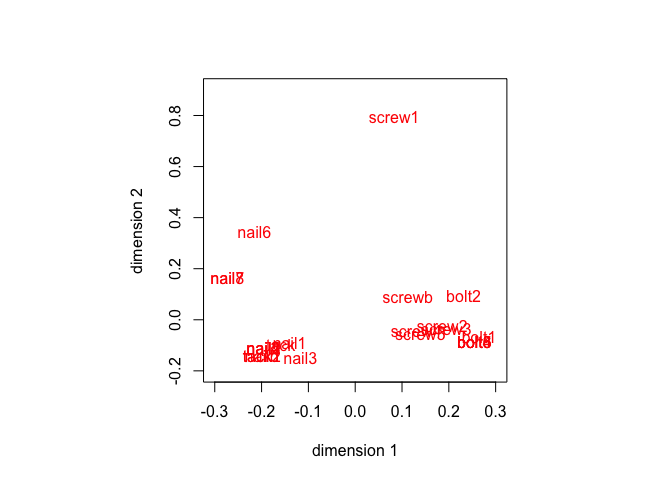
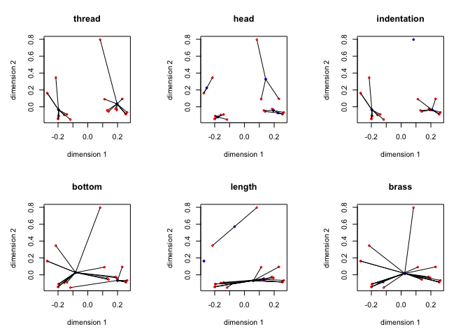
The star plots, produced by the utility
starPlotter() are in figure 3.
The discriminations matrices \(\Delta_j\) are
##      [,1]  [,2]
## [1,]  0.93  0.16
## [2,]  0.16  0.03
##      [,1]  [,2]
## [1,]  0.96  0.04
## [2,]  0.04  0.64
##      [,1]  [,2]
## [1,]  0.94  0.07
## [2,]  0.07  0.66
##      [,1]  [,2]
## [1,]  0.39 -0.13
## [2,] -0.13  0.04
##      [,1]  [,2]
## [1,]  0.29 -0.19
## [2,] -0.19  0.82
##      [,1]  [,2]
## [1,]  0.07  0.05
## [2,]  0.05  0.03
and their average \(\Lambda\) is
##      [,1]  [,2]
## [1,]  0.60  0.00
## [2,]  0.00  0.37
Note that the loss was 0.5157273, which is one minus the average of the trace of \(\Lambda\). The induced correlations are
##       [,1]  [,2]  [,3]  [,4]  [,5]  [,6]  [,7]  [,8]  [,9]
##  [1,]  1.00  1.00  0.01  0.98 -0.20  0.46  0.03  0.41 -0.22
##  [2,]  1.00  1.00 -0.00  0.98 -0.21  0.46  0.03  0.41 -0.22
##  [3,]  0.01 -0.00  1.00  0.08  0.38  0.18 -0.59  0.40 -0.02
##  [4,]  0.98  0.98  0.08  1.00  0.00  0.50 -0.10  0.43 -0.21
##  [5,] -0.20 -0.21  0.38  0.00  1.00  0.14 -0.66  0.05  0.09
##  [6,]  0.46  0.46  0.18  0.50  0.14  1.00 -0.17  0.28 -0.29
##  [7,]  0.03  0.03 -0.59 -0.10 -0.66 -0.17  1.00 -0.00 -0.10
##  [8,]  0.41  0.41  0.40  0.43  0.05  0.28 -0.00  1.00  0.23
##  [9,] -0.22 -0.22 -0.02 -0.21  0.09 -0.29 -0.10  0.23  1.00
Of the six variables, three are binary. Thus they only have a single transformed variable associated with them, which is just the standardization to mean zero and sum of squares one. The total number of transformed variables is consequently 9. The eigenvalues of the induced correlation matrix (divided by the number of variables, not the number of transformed variables) are
## [1] 0.60 0.37 0.21 0.13 0.10 0.07 0.02 0.00 0.00Note that the two dominant eigenvalues are again equal to the diagonal elements of \(\Lambda\).
7.3.2 GALO
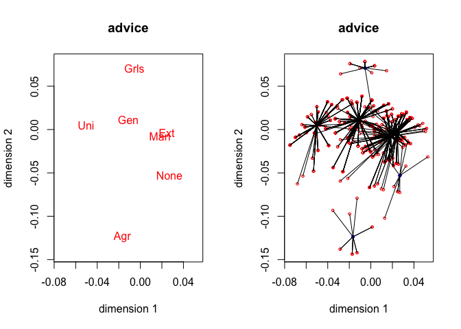
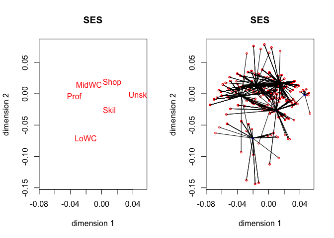
The second example is somewhat more realistic. In the GALO dataset (Peschar (1975)) data on 1290 school children in the sixth grade of an elementary school in 1959 in the city of Groningen (Netherlands) were collected. The variables are gender, IQ (categorized into 9 ordered categories), advice (teacher categorized the children into 7 possible forms of secondary education, i.e., Agr = agricultural; Ext = extended primary education; Gen = general; Grls = secondary school for girls; Man = manual, including housekeeping; None = no further education; Uni = pre- University), SES (parent’s profession in 6 categories) and school (37 different schools). The data have been analyzed previously in many Gifi publications, for example in De Leeuw and Mair (2009a). For our MCA we only make the first four variables, school is treated as passive
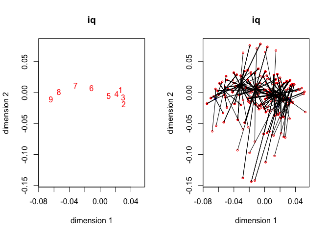
We use this example to illustrate some of the constraints on transformations. Two copies are used for all variables (although gender effectively only has one, of course). IQ is treated as ordinal, using a piecewise linear spline with knots at the nine data points.
galo_knots <- knotsD(galo)
galo_degrees <- c(-1,1,-1,-1,-1)
galo_ordinal <- c(FALSE, TRUE, FALSE, FALSE,FALSE)
galo_active <-c (TRUE, TRUE, TRUE, TRUE, FALSE)
h <- homals (galo, knots = galo_knots, degrees = galo_degrees, ordinal = galo_ordinal, active = galo_active)We first give transformations for the active variables (and their copies) in figure 4 . We skip gender, because transformation plots for binary variables are not very informative. We give two transformation plots for IQ, first using \(H\) and then using \(HA\). This illustrates the point made earlier, that transformation plots of block scores for ordinal variables with copies need not be monotone. It also illustrates that additional copies of an ordinal variable are not scaled to be monotone. Note that the plots for advice and SES are made with the utility stepPlotter(). Because the degree of the splines for those variables is zero, these transformation plots show step functions, with the steps at the knots, which are represented by vertical lines.
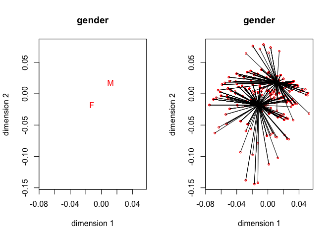
The four star plots for the active variables, together with the four category quantification plots, are in figure 5. Note that
homals() does not compute category quantifications, we have to compute them from the homals() output. Also note that for gender, advice and SES the object scores are connected to the category centroids of the variables. For IQ object scores are connected to points on the line connecting adjacent category quantifications. See De Leeuw and Van Rijckevorsel (1988) for category plots using forms of fuzzy coding (of which B-splines are an example).
For this analysis we need 52 iterations to obtain loss 0.54251. The average discrimination matrix over the four active variables is
##      [,1]  [,2]
## [1,]  0.54  0.00
## [2,]  0.00  0.38
while the eigenvalues of the induced correlation matrix of the active variables and their copies, divided by four, are
## [1] 0.54 0.38 0.26 0.21 0.18 0.13 0.05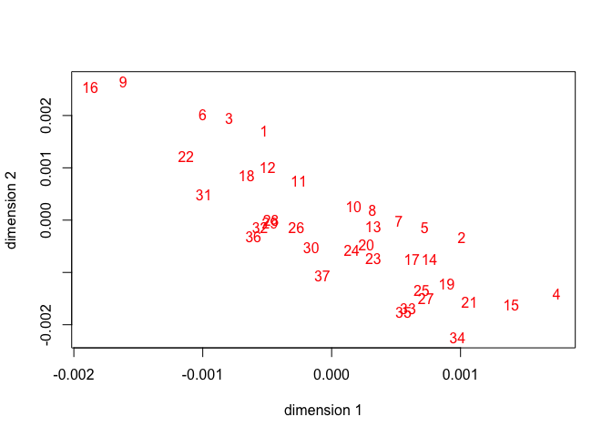
If we look at the scale of the plot we see all schools are pretty close to the origin. The discrimination matrices are consequently also small. In 1959 schools were pretty much the same.
##      [,1]    [,2]
## [1,]  0.0011 -0.0014
## [2,] -0.0014  0.0022
7.3.3 Thirteen Personality Scales
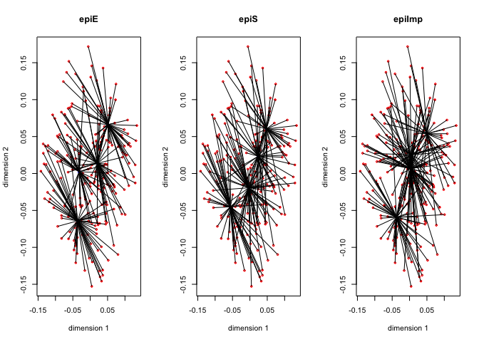
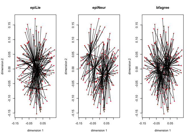
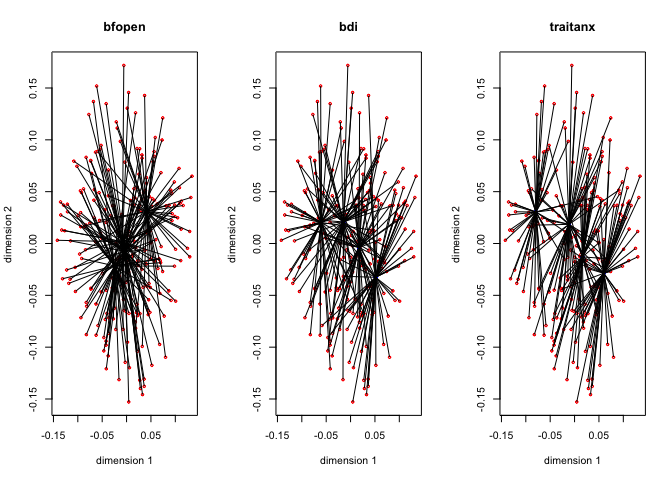
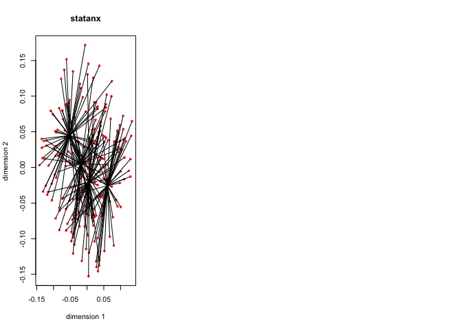
Our next example is a small data block from the psych package (Revelle 2015) of five scales from the Eysenck Personality Inventory, five from a Big Five inventory, a Beck Depression Inventory, and State and Trait Anxiety measures.
data(epi.bfi, package = "psych")
epi <- epi.bfi
epi_knots <- knotsQ(epi)
epi_degrees <- rep (0, 13)
epi_ordinal <- rep (FALSE, 13)
We perform a two-dimensional MCA, using degree zero and inner knots at the three quartiles for all 13 variables.
h <- homals(epi, knots = epi_knots, degrees = epi_degrees, ordinal = epi_ordinal)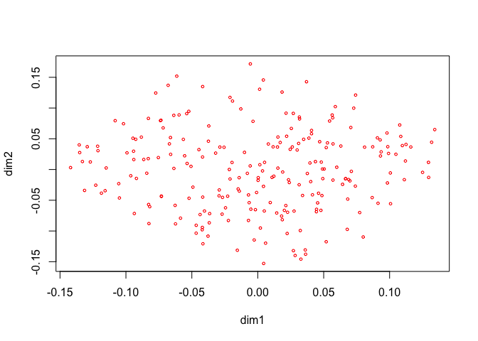
Figure 8 has the \(G_jY_j\) for each of the thirteen variables, with the first dimension in red, and the second dimension in blue.
The thirteen star plots are in figure 8.

Now change the degree to two for all variables, i.e. fit piecewise quadratic polynomials which are differentiable at the knots. We still have two copies for each variable, and these two copies define the blocks.
epi_degrees <- rep (2, 13)
h <- homals (epi, knots = epi_knots, degrees = epi_degrees, ordinal = epi_ordinal)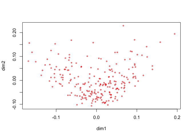
References
Hartigan, J. 1975. Clustering Algorithms. Wiley.
Gifi, A. 1990. Nonlinear Multivariate Analysis. New York, N.Y.: Wiley.
Peschar, J. L. 1975. School, Milieu, Beroep. Groningen, The Netherlands: Tjeek Willink.
De Leeuw, J., and P. Mair. 2009a. “Homogeneity Analysis in R: the Package homals.” Journal of Statistical Software 31 (4): 1–21. http://www.stat.ucla.edu/~deleeuw/janspubs/2009/articles/deleeuw_mair_A_09a.pdf.
De Leeuw, J., and J.L.A. Van Rijckevorsel. 1980. “HOMALS and Princals: Some Generalizations of Principal Components Analysis.” In Data Analysis and Informatics. Amsterdam: North Holland Publishing Company. http://www.stat.ucla.edu/~deleeuw/janspubs/1980/chapters/deleeuw_vanrijckevorsel_C_80.pdf.
1988. “Beyond Homogeneity Analysis.” In Component and Correspondence Analysis, edited by J.L.A. Van Rijckevorsel and J. De Leeuw, 55–80. Chichester, England: Wiley. http://www.stat.ucla.edu/~deleeuw/janspubs/1988/chapters/deleeuw_vanrijckevorsel_C_88.pdf.Revelle, William. 2015. Psych: Procedures for Psychological, Psychometric, and Personality Research. Evanston, Illinois: Northwestern University. http://CRAN.R-project.org/package=psych.