15 Discriminant Analysis and criminals()
15.1 Equations
If the second block contains more than one copy of a single variable and we use binary indicator coding for that variable, then we optimize the eigenvalue (between/within ratio) sums for a canonical discriminant analysis.
15.2 Examples
15.2.1 Iris data
The next example illustrates (canonical) discriminant analysis, using the obligatory Anderson-Fisher iris data. Since there are three species of iris, we use two copies for the species variable. The other four variables are in the same block, they are transformed using piecewise linear monotone splines with five knots.
data(iris, package="datasets")
iris_vars <- names(iris)
iris_knots <- knotsQ(iris[,1:4])
x <- as.matrix(iris[,1:4])
y <- as.matrix(iris[[5]])
h <- criminals (x, y, xdegrees = 1)In 191 iterations we find minimum loss 0.030226. The object scores are in figure 23 plotted against the original variables (not the transformed variables), and the transformation plots are in figure 24.
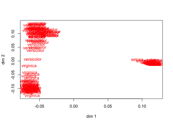
Discriminant analysis decomposes the total dispersion matrix \(T\) into a sum of a between-groups dispersion \(B\) and a within-groups dispersion \(W\), and then finds directions in the space spanned by the variables for which the between-variance is largest relative to the total variance. MVAOS optimizes the sum of the \(r\) largest eigenvalues of \(T^{-1}B\). Before optimal transformation these eigenvalues for the iris data are r, after transformation they are r.