Part 9 Week 4 Asynchronous
Data Visualization in R with ggplot2 > Week 1
9.1 Getting Started with ggplot Part 1, 2
library(tidyverse)

#####Load the data (if you want, you could do this locally from your computer rather than download from Dropbox)

cel <-
  read_csv(
    url(
      "https://www.dropbox.com/s/4ebgnkdhhxo5rac/cel_volden_wiseman%20_coursera.csv?raw=1"
    )
  )
#>
#> ── Column specification ─────────────────────────────────────────────
#> cols(
#> .default = col_double(),
#> thomas_name = col_character(),
#> st_name = col_character()
#> )
#> ℹ Use `spec()` for the full column specifications.names(cel)#> [1] "thomas_num" "thomas_name" "icpsr"
#> [4] "congress" "year" "st_name"
#> [7] "cd" "dem" "elected"
#> [10] "female" "votepct" "dwnom1"
#> [13] "deleg_size" "speaker" "subchr"
#> [16] "afam" "latino" "votepct_sq"
#> [19] "power" "chair" "state_leg"
#> [22] "state_leg_prof" "majority" "maj_leader"
#> [25] "min_leader" "meddist" "majdist"
#> [28] "all_bills" "all_aic" "all_abc"
#> [31] "all_pass" "all_law" "les"
#> [34] "seniority" "benchmark" "expectation"
#> [37] "TotalInParty" "RankInParty"dim(cel)#> [1] 10262 38table(cel$year)#>
#> 1973 1975 1977 1979 1981 1983 1985 1987 1989 1991 1993 1995 1997
#> 444 444 443 442 447 444 445 446 449 447 446 445 449
#> 1999 2001 2003 2005 2007 2009 2011 2013 2015 2017
#> 442 447 444 445 452 451 449 450 443 448summary(cel$all_bills)#> Min. 1st Qu. Median Mean 3rd Qu. Max.
#> 0.0 7.0 12.0 16.8 21.0 258.0#for making a scatterplot
####filter the data we want
fig115 <- filter(cel, congress == 115)
fig115 <- select(fig115, "seniority", "all_pass")
####these commands do the same thing as above, just with piping
fig115 <-
cel %>% filter(congress == 115) %>% select("seniority", "all_pass")
###check to make sure the filter worked properly
head(fig115)#> # A tibble: 6 x 2
#> seniority all_pass
#> <dbl> <dbl>
#> 1 2 1
#> 2 3 2
#> 3 11 0
#> 4 2 3
#> 5 2 1
#> 6 4 1####set up the data and aesthetics
ggplot(fig115, aes(x = seniority, y = all_pass))
####add the marks
ggplot(fig115, aes(x = seniority, y = all_pass)) +
  geom_point()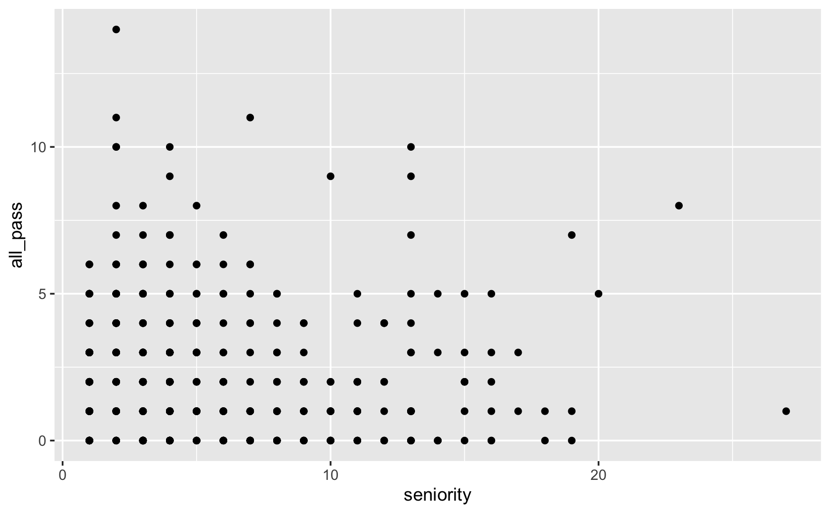
####jitter adds random noise to the data to avoid overplotting
ggplot(fig115, aes(x = seniority, y = all_pass)) +
  geom_jitter()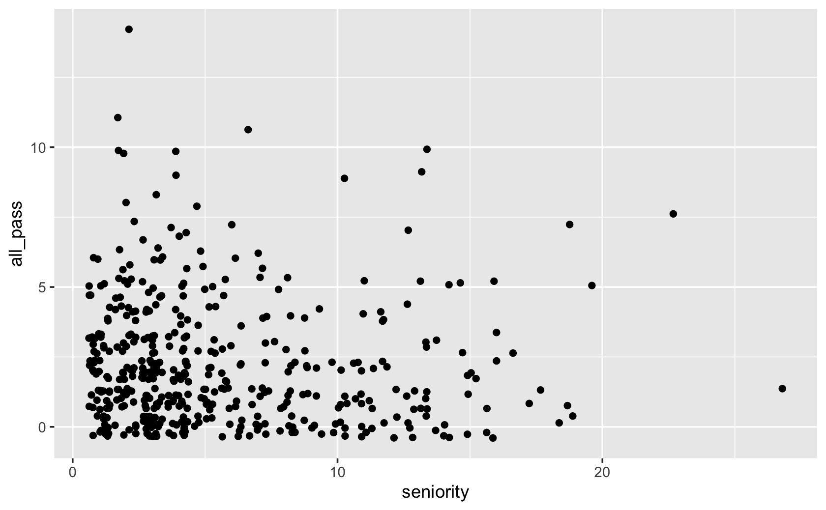
####add some labels and a title
ggplot(fig115, aes(x = seniority, y = all_pass)) +
  geom_jitter() +
  labs(x = "Seniority", y = "Bills Passed", title = "Seniority and Bills Passed in the 115th Congress")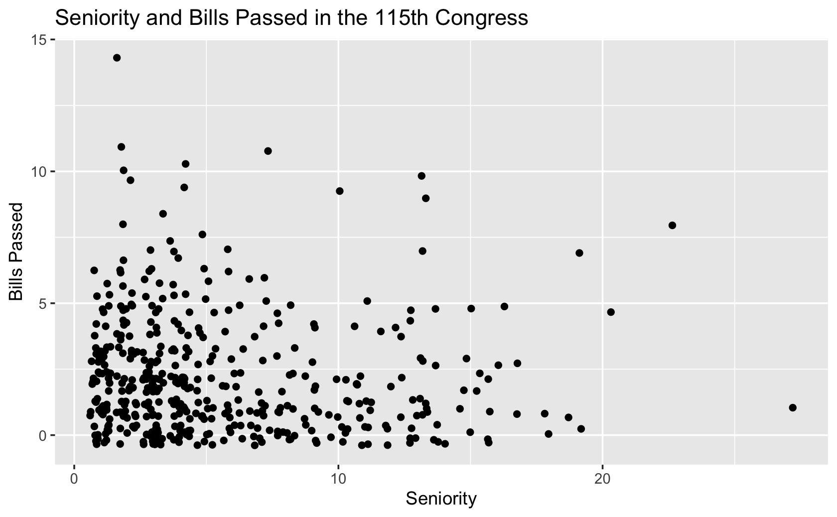
#####modify filter and select to grab "dem"

fig115 <- cel %>%
  filter(congress == 115) %>%
  select("seniority", "all_pass", "dem")

fig115$dem
#> [1] 0 1 0 1 0 0 0 0 0 0 0 0 0 1 0 1 1 1 0 1 0 0 0 0 1 0 0 0 1 1 1 1
#> [33] 0 1 0 1 0 0 0 0 1 1 0 0 0 0 0 1 1 0 0 1 1 1 1 0 0 1 1 1 0 0 0 1
#> [65] 1 1 1 1 1 1 0 1 0 0 0 0 0 0 1 1 0 1 1 1 0 1 0 0 1 1 1 0 1 0 0 0
#> [97] 1 0 1 1 1 1 0 1 1 1 1 0 0 0 1 0 1 1 0 1 0 0 0 0 1 0 1 1 1 0 1 1
#> [129] 0 0 0 0 0 0 0 1 0 1 0 0 1 1 0 0 1 1 0 0 0 0 1 1 0 0 0 1 0 0 0 0
#> [161] 0 1 1 0 1 0 0 1 1 0 0 0 0 1 1 0 0 0 1 0 0 1 0 0 1 0 1 0 0 0 0 0
#> [193] 1 1 1 0 0 0 1 1 0 0 1 0 0 0 1 0 1 0 1 0 1 1 1 1 1 1 0 0 0 0 1 1
#> [225] 0 0 0 0 1 0 0 1 1 1 0 1 1 1 0 1 0 1 1 1 0 1 1 0 0 0 1 1 0 0 1 1
#> [257] 1 0 1 1 0 0 0 0 0 1 0 0 0 1 1 1 0 0 0 1 0 0 0 1 1 0 0 0 0 1 1 1
#> [289] 0 1 0 1 1 1 0 0 1 1 0 1 0 1 1 0 0 1 0 1 1 0 1 0 1 1 0 1 1 1 0 1
#> [321] 1 0 0 1 0 1 1 0 1 0 0 0 0 1 0 1 0 0 0 0 0 0 0 0 0 1 0 0 0 0 1 0
#> [353] 1 1 1 0 0 0 1 1 1 0 1 0 1 1 1 1 1 0 0 1 1 0 1 0 1 1 1 0 0 0 1 1
#> [385] 1 1 0 0 0 0 0 1 1 0 0 0 1 1 1 0 0 1 0 1 0 0 0 1 1 1 0 1 0 0 0 1
#> [417] 1 1 1 1 0 0 0 0 0 0 1 1 1 1 0 0 1 0 0 1 0 1 0 0 0 0 1 0 0 0 0 0ggplot(fig115, aes(x = seniority, y = all_pass, color = dem)) +
geom_jitter() +
labs(x = "Seniority", y = "Bills Passed", title = "Seniority and Bills Passed in the 115th Congress")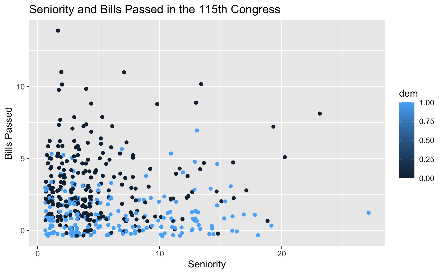
####colors are strange, let's fix

#####make dem a categorical variable called "party"
party <- recode(fig115$dem, `1` = "Democrat", `0` = "Republican")

fig115 <- add_column(fig115, party)

fig115$party
#> [1] "Republican" "Democrat" "Republican" "Democrat"
#> [5] "Republican" "Republican" "Republican" "Republican"
#> [9] "Republican" "Republican" "Republican" "Republican"
#> [13] "Republican" "Democrat" "Republican" "Democrat"
#> [17] "Democrat" "Democrat" "Republican" "Democrat"
#> [21] "Republican" "Republican" "Republican" "Republican"
#> [25] "Democrat" "Republican" "Republican" "Republican"
#> [29] "Democrat" "Democrat" "Democrat" "Democrat"
#> [33] "Republican" "Democrat" "Republican" "Democrat"
#> [37] "Republican" "Republican" "Republican" "Republican"
#> [41] "Democrat" "Democrat" "Republican" "Republican"
#> [45] "Republican" "Republican" "Republican" "Democrat"
#> [49] "Democrat" "Republican" "Republican" "Democrat"
#> [53] "Democrat" "Democrat" "Democrat" "Republican"
#> [57] "Republican" "Democrat" "Democrat" "Democrat"
#> [61] "Republican" "Republican" "Republican" "Democrat"
#> [65] "Democrat" "Democrat" "Democrat" "Democrat"
#> [69] "Democrat" "Democrat" "Republican" "Democrat"
#> [73] "Republican" "Republican" "Republican" "Republican"
#> [77] "Republican" "Republican" "Democrat" "Democrat"
#> [81] "Republican" "Democrat" "Democrat" "Democrat"
#> [85] "Republican" "Democrat" "Republican" "Republican"
#> [89] "Democrat" "Democrat" "Democrat" "Republican"
#> [93] "Democrat" "Republican" "Republican" "Republican"
#> [97] "Democrat" "Republican" "Democrat" "Democrat"
#> [101] "Democrat" "Democrat" "Republican" "Democrat"
#> [105] "Democrat" "Democrat" "Democrat" "Republican"
#> [109] "Republican" "Republican" "Democrat" "Republican"
#> [113] "Democrat" "Democrat" "Republican" "Democrat"
#> [117] "Republican" "Republican" "Republican" "Republican"
#> [121] "Democrat" "Republican" "Democrat" "Democrat"
#> [125] "Democrat" "Republican" "Democrat" "Democrat"
#> [129] "Republican" "Republican" "Republican" "Republican"
#> [133] "Republican" "Republican" "Republican" "Democrat"
#> [137] "Republican" "Democrat" "Republican" "Republican"
#> [141] "Democrat" "Democrat" "Republican" "Republican"
#> [145] "Democrat" "Democrat" "Republican" "Republican"
#> [149] "Republican" "Republican" "Democrat" "Democrat"
#> [153] "Republican" "Republican" "Republican" "Democrat"
#> [157] "Republican" "Republican" "Republican" "Republican"
#> [161] "Republican" "Democrat" "Democrat" "Republican"
#> [165] "Democrat" "Republican" "Republican" "Democrat"
#> [169] "Democrat" "Republican" "Republican" "Republican"
#> [173] "Republican" "Democrat" "Democrat" "Republican"
#> [177] "Republican" "Republican" "Democrat" "Republican"
#> [181] "Republican" "Democrat" "Republican" "Republican"
#> [185] "Democrat" "Republican" "Democrat" "Republican"
#> [189] "Republican" "Republican" "Republican" "Republican"
#> [193] "Democrat" "Democrat" "Democrat" "Republican"
#> [197] "Republican" "Republican" "Democrat" "Democrat"
#> [201] "Republican" "Republican" "Democrat" "Republican"
#> [205] "Republican" "Republican" "Democrat" "Republican"
#> [209] "Democrat" "Republican" "Democrat" "Republican"
#> [213] "Democrat" "Democrat" "Democrat" "Democrat"
#> [217] "Democrat" "Democrat" "Republican" "Republican"
#> [221] "Republican" "Republican" "Democrat" "Democrat"
#> [225] "Republican" "Republican" "Republican" "Republican"
#> [229] "Democrat" "Republican" "Republican" "Democrat"
#> [233] "Democrat" "Democrat" "Republican" "Democrat"
#> [237] "Democrat" "Democrat" "Republican" "Democrat"
#> [241] "Republican" "Democrat" "Democrat" "Democrat"
#> [245] "Republican" "Democrat" "Democrat" "Republican"
#> [249] "Republican" "Republican" "Democrat" "Democrat"
#> [253] "Republican" "Republican" "Democrat" "Democrat"
#> [257] "Democrat" "Republican" "Democrat" "Democrat"
#> [261] "Republican" "Republican" "Republican" "Republican"
#> [265] "Republican" "Democrat" "Republican" "Republican"
#> [269] "Republican" "Democrat" "Democrat" "Democrat"
#> [273] "Republican" "Republican" "Republican" "Democrat"
#> [277] "Republican" "Republican" "Republican" "Democrat"
#> [281] "Democrat" "Republican" "Republican" "Republican"
#> [285] "Republican" "Democrat" "Democrat" "Democrat"
#> [289] "Republican" "Democrat" "Republican" "Democrat"
#> [293] "Democrat" "Democrat" "Republican" "Republican"
#> [297] "Democrat" "Democrat" "Republican" "Democrat"
#> [301] "Republican" "Democrat" "Democrat" "Republican"
#> [305] "Republican" "Democrat" "Republican" "Democrat"
#> [309] "Democrat" "Republican" "Democrat" "Republican"
#> [313] "Democrat" "Democrat" "Republican" "Democrat"
#> [317] "Democrat" "Democrat" "Republican" "Democrat"
#> [321] "Democrat" "Republican" "Republican" "Democrat"
#> [325] "Republican" "Democrat" "Democrat" "Republican"
#> [329] "Democrat" "Republican" "Republican" "Republican"
#> [333] "Republican" "Democrat" "Republican" "Democrat"
#> [337] "Republican" "Republican" "Republican" "Republican"
#> [341] "Republican" "Republican" "Republican" "Republican"
#> [345] "Republican" "Democrat" "Republican" "Republican"
#> [349] "Republican" "Republican" "Democrat" "Republican"
#> [353] "Democrat" "Democrat" "Democrat" "Republican"
#> [357] "Republican" "Republican" "Democrat" "Democrat"
#> [361] "Democrat" "Republican" "Democrat" "Republican"
#> [365] "Democrat" "Democrat" "Democrat" "Democrat"
#> [369] "Democrat" "Republican" "Republican" "Democrat"
#> [373] "Democrat" "Republican" "Democrat" "Republican"
#> [377] "Democrat" "Democrat" "Democrat" "Republican"
#> [381] "Republican" "Republican" "Democrat" "Democrat"
#> [385] "Democrat" "Democrat" "Republican" "Republican"
#> [389] "Republican" "Republican" "Republican" "Democrat"
#> [393] "Democrat" "Republican" "Republican" "Republican"
#> [397] "Democrat" "Democrat" "Democrat" "Republican"
#> [401] "Republican" "Democrat" "Republican" "Democrat"
#> [405] "Republican" "Republican" "Republican" "Democrat"
#> [409] "Democrat" "Democrat" "Republican" "Democrat"
#> [413] "Republican" "Republican" "Republican" "Democrat"
#> [417] "Democrat" "Democrat" "Democrat" "Democrat"
#> [421] "Republican" "Republican" "Republican" "Republican"
#> [425] "Republican" "Republican" "Democrat" "Democrat"
#> [429] "Democrat" "Democrat" "Republican" "Republican"
#> [433] "Democrat" "Republican" "Republican" "Democrat"
#> [437] "Republican" "Democrat" "Republican" "Republican"
#> [441] "Republican" "Republican" "Democrat" "Republican"
#> [445] "Republican" "Republican" "Republican" "Republican"ggplot(fig115, aes(x = seniority, y = all_pass, color = party)) +
geom_jitter() +
labs(x = "Seniority", y = "Bills Passed", title = "Seniority and Bills Passed in the 115th Congress")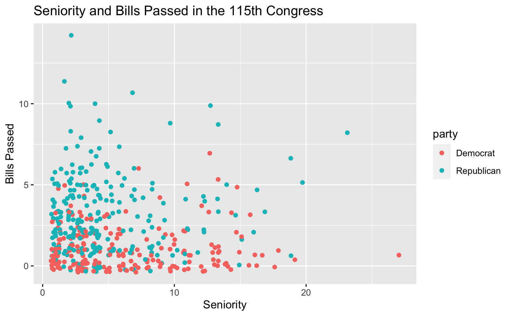
####let's make the colors match traditional blue democrats and red republicans
ggplot(fig115, aes(x = seniority, y = all_pass, color = party)) +
  geom_jitter() +
labs(x = "Seniority", y = "Bills Passed", title = "Seniority and Bills Passed in the 115th Congress") +
scale_color_manual(values = c("blue", "red"))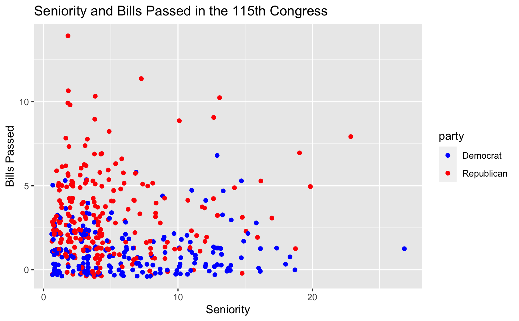
#####make two separate plots using facet_wrap

ggplot(fig115, aes(x = seniority, y = all_pass, color = party)) +
  geom_jitter() +
  labs(x = "Seniority", y = "Bills Passed", title = "Seniority and Bills Passed in the 115th Congress") +
  scale_color_manual(values = c("blue", "red")) +
  facet_wrap( ~ party)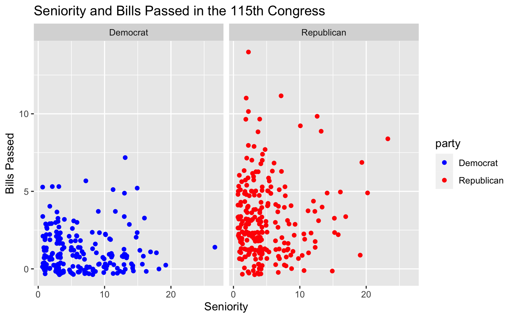
9.2 Distributions
library(tidyverse)

cces <- read_csv("week4/cces.csv")
#>
#> ── Column specification ─────────────────────────────────────────────
#> cols(
#> .default = col_double()
#> )
#> ℹ Use `spec()` for the full column specifications.#####boxplots
###make a basic boxplot
ggplot(cces, aes(y = faminc_new)) + geom_boxplot()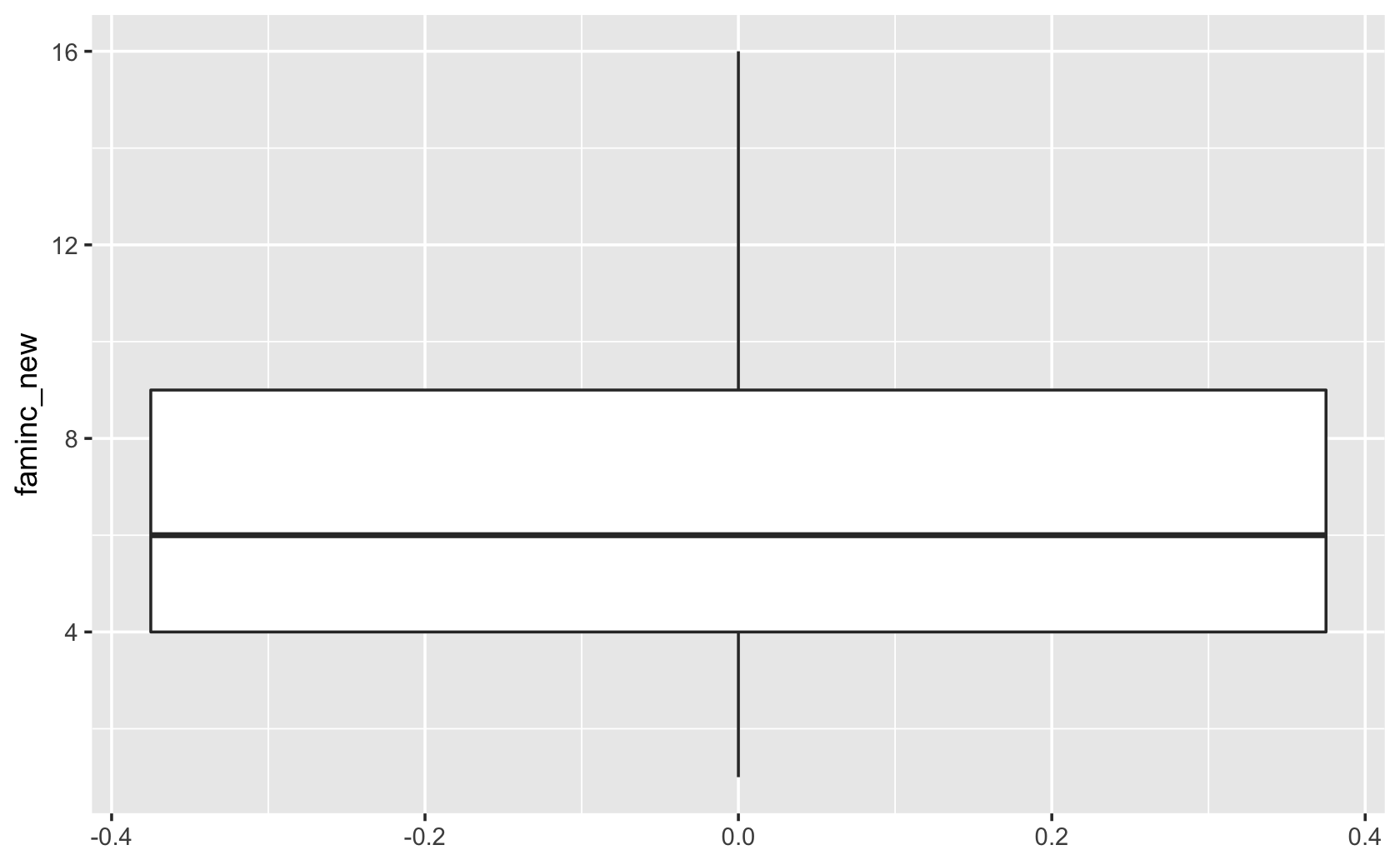
####break up boxplots by education group -- add a aesthetic mapping for group
ggplot(cces, aes(y = faminc_new, group = educ)) +
  geom_boxplot()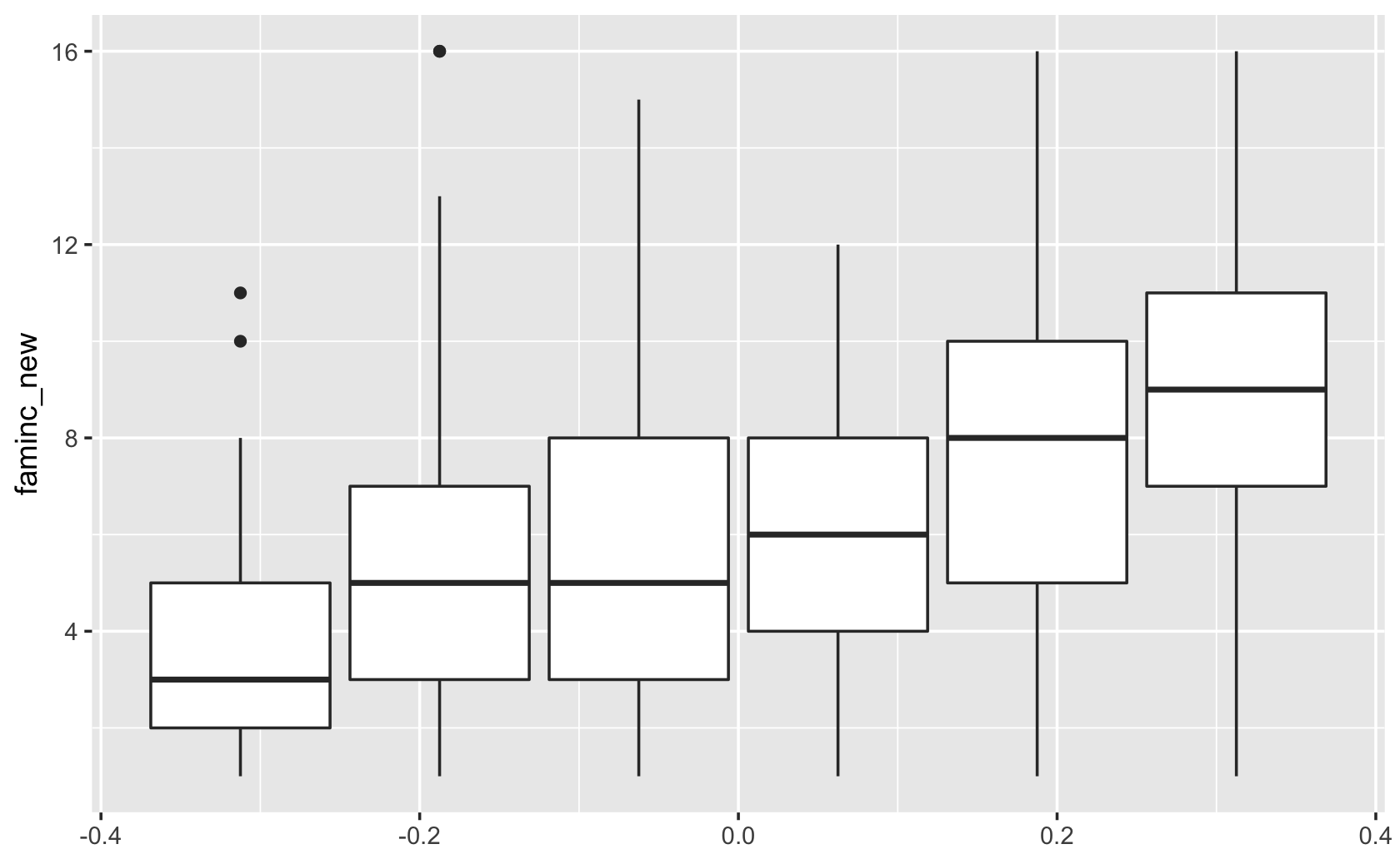
####add labels and a title
ggplot(cces, aes(y = faminc_new, group = educ)) +
  geom_boxplot() +
  labs(x = "Income Level", y = "Family Income", title = "Family Inc. by Respondent Ed. Level")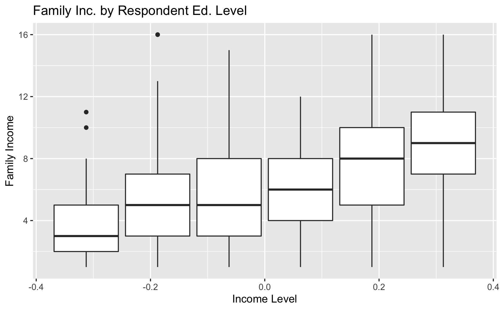
####reformat the data to create a dichotomous categorical variable for four-year college grads or more, and then all respondents with 2 year college degrees or less

cces$educ_category <-
  recode(
    cces$educ,
    `1` = "<4 yr Degree",
    `2` = "<4 yr Degree",
    `3` = "<4 yr Degree",
    `4` = "<4 yr Degree",
    `5` = "4 yr Deg. +",
    `6` = "4 yr Deg. +"
  )

###make sure you change the aesthetic mapping so the new categorical variable is mapped to "x" rather than "group"

ggplot(cces, aes(y = faminc_new, x = educ_category)) +
  geom_boxplot() +
  labs(x = "Income Level", y = "Family Income", title = "Family Inc. by Respondent Ed. Level")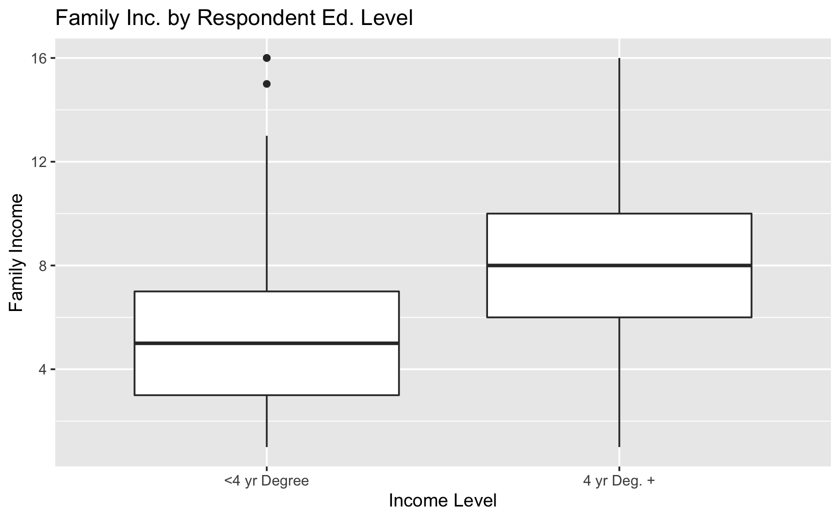
####make a histogram
ggplot(cces, aes(x = faminc_new)) +
  geom_histogram()
#> `stat_bin()` using `bins = 30`. Pick better value with `binwidth`.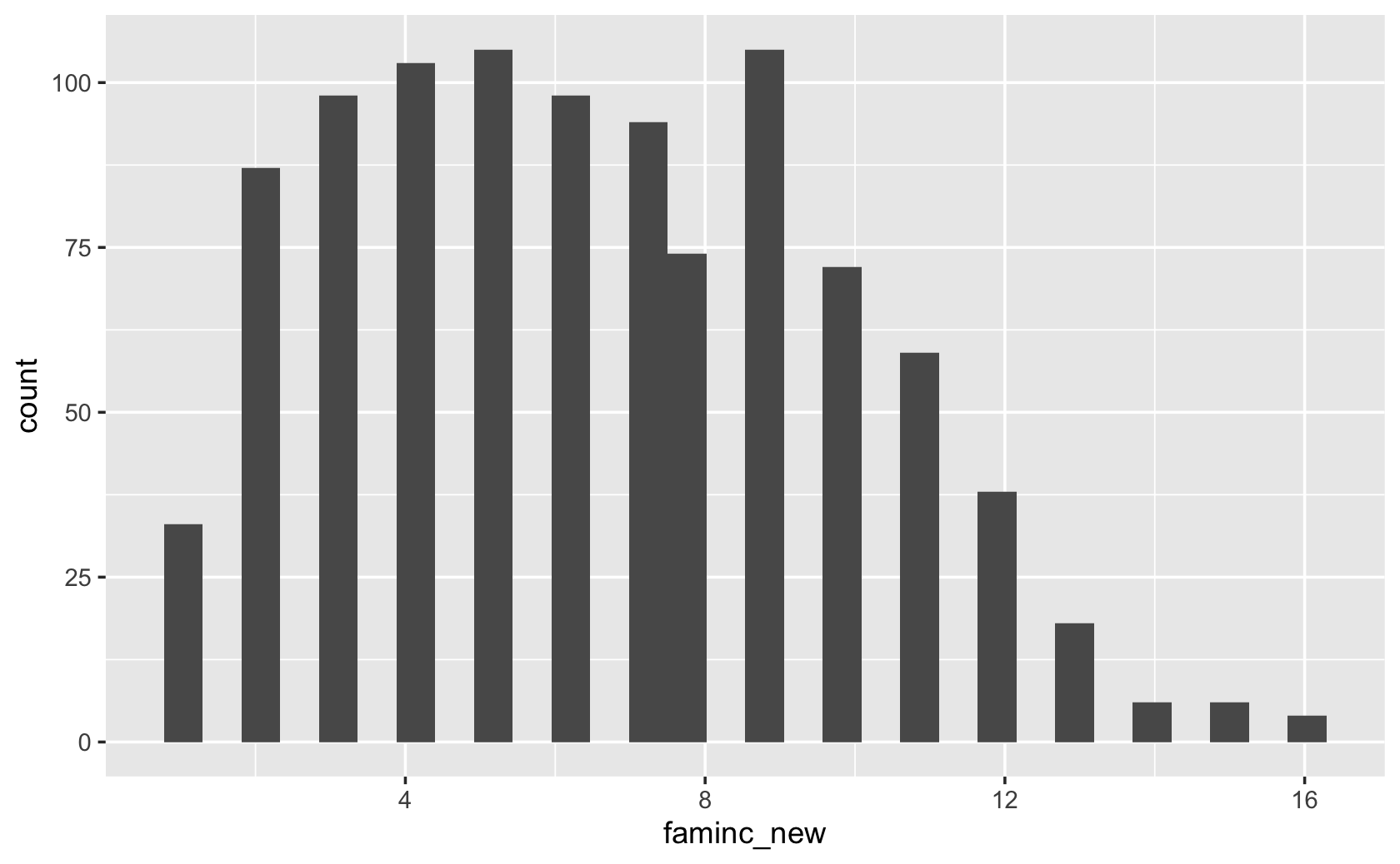
####make a density plot
ggplot(cces, aes(x = faminc_new)) +
  geom_density()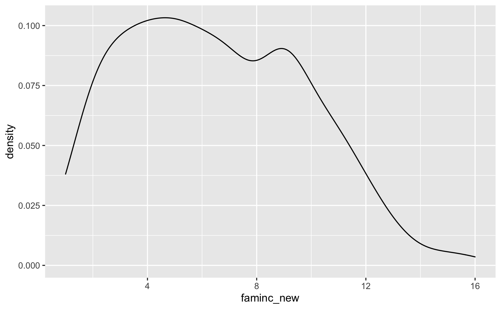
9.3 Practices for week 4
######DO NOT MODIFY. This will load required packages and data.
library(tidyverse)
cel <- drop_na(read_csv(url("https://www.dropbox.com/s/4ebgnkdhhxo5rac/cel_volden_wiseman%20_coursera.csv?raw=1")))
#>
#> ── Column specification ─────────────────────────────────────────────
#> cols(
#> .default = col_double(),
#> thomas_name = col_character(),
#> st_name = col_character()
#> )
#> ℹ Use `spec()` for the full column specifications.Your objective is to replicate these figures, created using the Center of Legislative Effectiveness Data. These figures are similar to those we completed in the lecture videos.
IMPORTANT: Filter your data so you are only displaying information for the 115th Congress.
cel %>% glimpse()#> Rows: 9,845
#> Columns: 38
#> $ thomas_num <dbl> 1, 2, 3, 4, 6, 8, 7, 9, 10, 11, 12, 14, 15, …
#> $ thomas_name <chr> "Abdnor, James", "Abzug, Bella", "Adams, Bro…
#> $ icpsr <dbl> 14000, 13001, 10700, 10500, 12000, 12001, 10…
#> $ congress <dbl> 93, 93, 93, 93, 93, 93, 93, 93, 93, 93, 93, …
#> $ year <dbl> 1973, 1973, 1973, 1973, 1973, 1973, 1973, 19…
#> $ st_name <chr> "SD", "NY", "WA", "NY", "AR", "CA", "IL", "N…
#> $ cd <dbl> 2, 20, 7, 7, 1, 35, 16, 4, 1, 11, 7, 5, 17, …
#> $ dem <dbl> 0, 1, 1, 1, 1, 1, 0, 1, 0, 1, 0, 0, 0, 1, 1,…
#> $ elected <dbl> 1972, 1970, 1964, 1960, 1968, 1968, 1960, 19…
#> $ female <dbl> 0, 1, 0, 0, 0, 0, 0, 0, 0, 0, 0, 0, 0, 0, 0,…
#> $ votepct <dbl> 55, 56, 85, 75, 100, 75, 72, 50, 73, 53, 82,…
#> $ dwnom1 <dbl> 0.228, -0.687, -0.361, -0.400, -0.281, -0.29…
#> $ deleg_size <dbl> 6, 39, 7, 39, 4, 43, 24, 11, 1, 24, 24, 5, 2…
#> $ speaker <dbl> 0, 0, 0, 0, 0, 0, 0, 0, 0, 0, 0, 0, 0, 0, 0,…
#> $ subchr <dbl> 0, 0, 1, 1, 1, 0, 0, 0, 0, 1, 0, 0, 0, 1, 0,…
#> $ afam <dbl> 0, 0, 0, 0, 0, 0, 0, 0, 0, 0, 0, 0, 0, 0, 0,…
#> $ latino <dbl> 0, 0, 0, 0, 0, 0, 0, 0, 0, 0, 0, 0, 0, 0, 0,…
#> $ votepct_sq <dbl> 3025, 3136, 7225, 5625, 10000, 5625, 5184, 2…
#> $ power <dbl> 0, 0, 0, 1, 0, 0, 1, 0, 1, 0, 1, 0, 0, 0, 0,…
#> $ chair <dbl> 0, 0, 0, 0, 0, 0, 0, 0, 0, 0, 0, 0, 0, 0, 0,…
#> $ state_leg <dbl> 1, 0, 0, 0, 0, 1, 0, 1, 0, 0, 1, 1, 1, 0, 0,…
#> $ state_leg_prof <dbl> 0.104, 0.000, 0.000, 0.000, 0.000, 0.526, 0.…
#> $ majority <dbl> 0, 1, 1, 1, 1, 1, 0, 1, 0, 1, 0, 0, 0, 1, 1,…
#> $ maj_leader <dbl> 0, 0, 0, 0, 0, 0, 0, 0, 0, 0, 0, 0, 0, 0, 0,…
#> $ min_leader <dbl> 0, 0, 0, 0, 0, 0, 1, 0, 0, 0, 0, 0, 0, 0, 0,…
#> $ meddist <dbl> 0.275, 0.640, 0.314, 0.353, 0.234, 0.246, 0.…
#> $ majdist <dbl> 0.5475, 0.3675, 0.0415, 0.0805, 0.0385, 0.02…
#> $ all_bills <dbl> 22, 136, 37, 38, 53, 87, 55, 17, 23, 53, 35,…
#> $ all_aic <dbl> 0, 1, 2, 0, 3, 0, 0, 0, 0, 2, 0, 1, 0, 5, 0,…
#> $ all_abc <dbl> 0, 1, 2, 0, 3, 0, 0, 0, 0, 2, 0, 1, 0, 5, 0,…
#> $ all_pass <dbl> 0, 1, 2, 0, 2, 0, 0, 0, 0, 2, 0, 1, 0, 5, 0,…
#> $ all_law <dbl> 0, 1, 1, 0, 1, 0, 0, 0, 0, 1, 0, 1, 0, 2, 0,…
#> $ les <dbl> 0.10957, 0.76243, 1.23648, 0.15505, 1.87505,…
#> $ seniority <dbl> 1, 2, 5, 7, 3, 3, 7, 1, 6, 5, 2, 1, 7, 10, 2…
#> $ benchmark <dbl> 0.2713, 0.5108, 1.5303, 1.5845, 1.4762, 0.53…
#> $ expectation <dbl> 1, 2, 2, 1, 2, 2, 2, 1, 1, 1, 2, 2, 1, 3, 2,…
#> $ TotalInParty <dbl> 197, 248, 248, 248, 248, 248, 197, 248, 197,…
#> $ RankInParty <dbl> 132, 119, 88, 197, 64, 147, 67, 218, 135, 12…cel %>%
select(congress) %>%
unique()#> # A tibble: 23 x 1
#> congress
#> <dbl>
#> 1 93
#> 2 94
#> 3 95
#> 4 96
#> 5 97
#> 6 98
#> # … with 17 more rowsdf <- cel %>%
filter(congress == 115)
df#> # A tibble: 442 x 38
#> thomas_num thomas_name icpsr congress year st_name cd dem
#> <dbl> <chr> <dbl> <dbl> <dbl> <chr> <dbl> <dbl>
#> 1 9807 Abraham, Ralph 21522 115 2017 LA 5 0
#> 2 9808 Adams, Alma 21545 115 2017 NC 12 1
#> 3 9809 Aderholt, Robe… 29701 115 2017 AL 4 0
#> 4 9810 Aguilar, Pete 21506 115 2017 CA 31 1
#> 5 9811 Allen, Rick 21516 115 2017 GA 12 0
#> 6 9812 Amash, Justin 21143 115 2017 MI 3 0
#> # … with 436 more rows, and 30 more variables: elected <dbl>,
#> # female <dbl>, votepct <dbl>, dwnom1 <dbl>, deleg_size <dbl>,
#> # speaker <dbl>, subchr <dbl>, afam <dbl>, latino <dbl>,
#> # votepct_sq <dbl>, power <dbl>, chair <dbl>, state_leg <dbl>,
#> # state_leg_prof <dbl>, majority <dbl>, maj_leader <dbl>,
#> # min_leader <dbl>, meddist <dbl>, majdist <dbl>, all_bills <dbl>,
#> # all_aic <dbl>, all_abc <dbl>, all_pass <dbl>, all_law <dbl>,
#> # les <dbl>, seniority <dbl>, benchmark <dbl>, expectation <dbl>,
#> # TotalInParty <dbl>, RankInParty <dbl>9.3.1 Exercise 1
Hints:
For the y-axis, use the variable “all_pass.”
For the x-axis, use the variable “dwnom1.”
Make sure you recode the data for the “female” variable and rename it as “Gender” to generate the correct labels for the legend.
Set the color aesthetic in the ggplot() function to make the color of the dots change based on Gender.
Make sure the axis labels are correct.
# Use recode()
df_recode <- df
df_recode$female <- df_recode$female %>%
  recode(`1` = "Female",
         `0` = "Male")

df_recode %>%
  ggplot(aes(y = all_pass, x = dwnom1, color = female)) +
  geom_point() +
  labs(x = "Ideology", y = "Bills Passed", color = "Gender")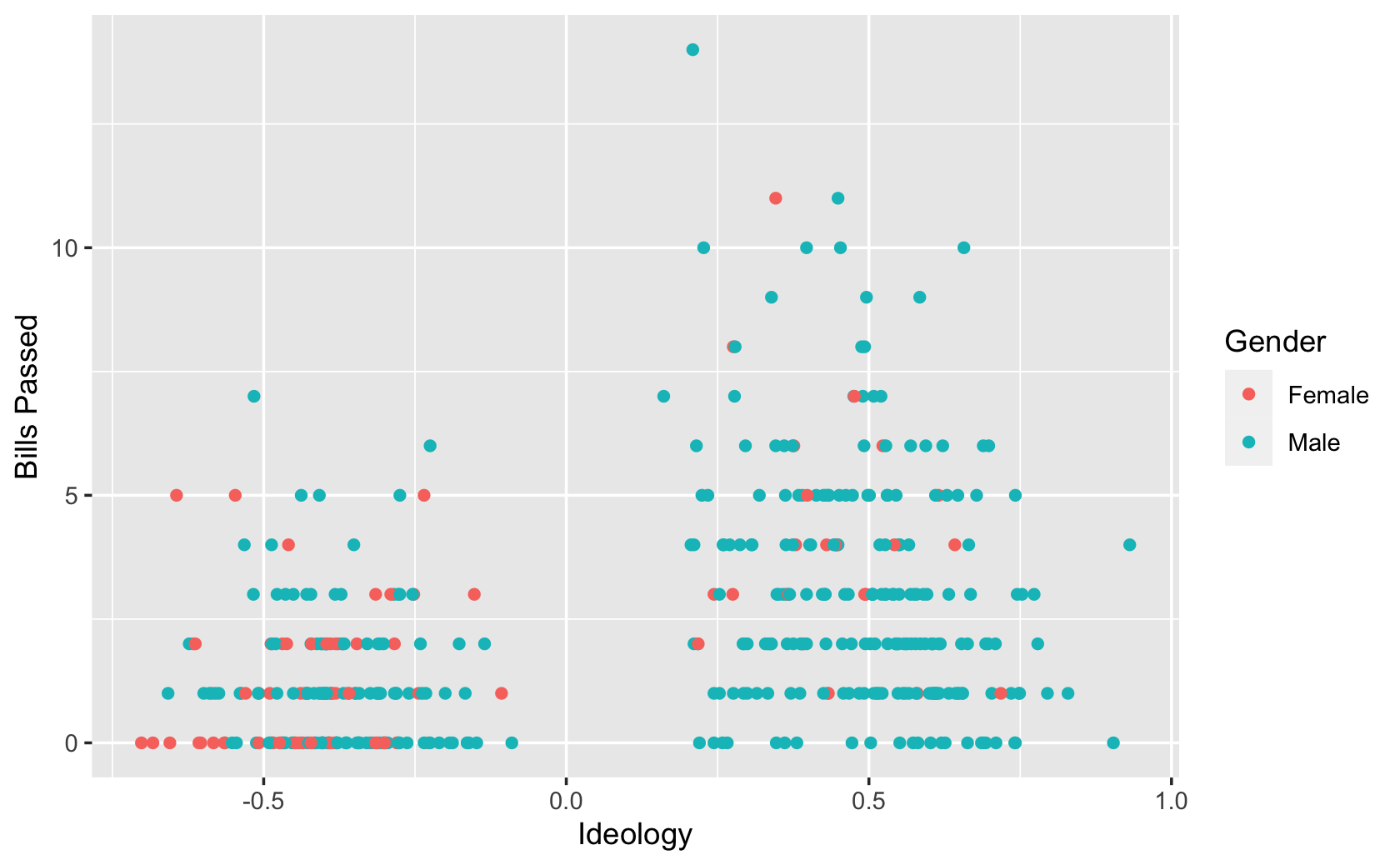
df %>%
  mutate(
    Gender = case_when(
      female == 1 ~ "Female",
      female == 0 ~ "Male"
  )) %>%
  ggplot(aes(y = all_pass, x = dwnom1, color = Gender)) +
  geom_point() +
  labs(x = "Ideology", y = "Bills Passed")
df %>%
  mutate(Gender = case_when(
    female == 1 ~ "Female",
    female == 0 ~ "Male"
  )) %>%
  ggplot(aes(y = all_pass, x = dwnom1, color = Gender)) +
  geom_jitter(alpha = 0.5) + # jitter adds random noise to the data to avoid overplotting
  labs(x = "Ideology", y = "Bills Passed")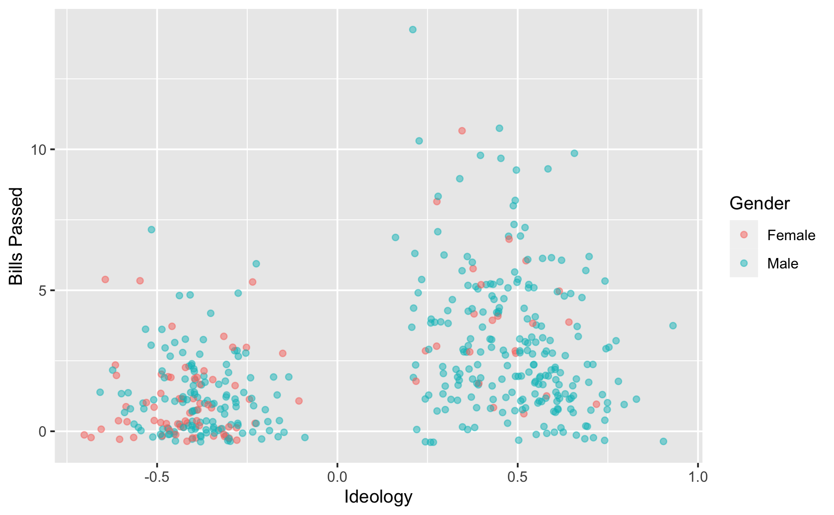
9.3.2 Exercise 2
Hints:
For the x-axis, use the variable “votepct.”
For the y-axis, use “all_pass.”
Make sure you recode the data for the “female” variable to generate the correct labels for the legend. Rename that column “Gender.” (you may have already done this in the last exercise)
Make sure you recode the data for “majority” variable to generate the correct labels of the facetted figures.
Set the color aesthetic in the ggplot() function to make the color of the dots change based on Gender.
Use scale_color_manual() to set the colors to green for males and orange for females.
Make sure the axis labels are correct.
# Use recode()
df_recode$majority <- df_recode$majority %>%
  recode(`1` = "Majority",
         `0` = "Minority")

df_recode %>%
  ggplot(aes(x = votepct, y = all_pass, color = female)) +
  geom_point() +
  facet_wrap( ~ majority) +
  scale_color_manual(values = c("orange", "green")) +
  labs(x = "Vote Percentage", y = "Bills Passed", color = "Gender")
####PUT YOUR CODE HERE
df %>%
  mutate(
    Gender = case_when(
      female == 1 ~ "Female",
      female == 0 ~ "Male"
    ),
    majority_minority = case_when(
      majority == 1 ~ "Majority",
      majority == 0 ~ "Minority"
    )
  ) %>%
  ggplot(aes(x = votepct, y = all_pass, color = Gender)) +
  geom_point() +
  facet_wrap( ~ majority_minority) +
  scale_color_manual(values = c("orange", "green")) +
  labs(x = "Vote Percentage", y = "Bills Passed")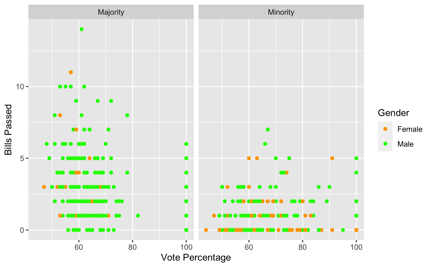
df %>%
  mutate(
    Gender = case_when(
      female == 1 ~ "Female",
      female == 0 ~ "Male"
    ),
    majority_minority = case_when(
      majority == 1 ~ "Majority",
      majority == 0 ~ "Minority"
    )
  ) %>%
  ggplot(aes(x = votepct, y = all_pass, color = Gender)) +
  geom_jitter(alpha = 0.5) +
  facet_wrap( ~ majority_minority) +
  scale_color_manual(values = c("orange", "green")) +
  labs(x = "Vote Percentage", y = "Bills Passed")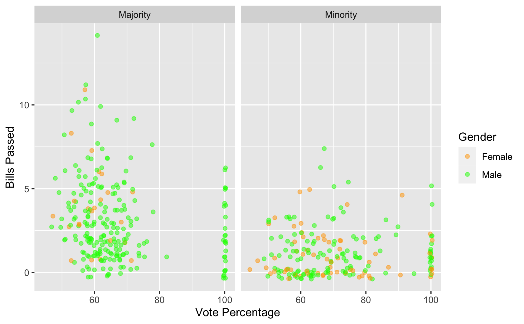
9.3.3 Exercise 3
Hints:
For the y-axis, use the variable “les.”
Make sure you recode the data for the “majority” variable to generate the correct labels. (you may have already done this in the last exercise)
Make sure the axis labels and figure title are correct.
# Use recode()
df_recode %>%
  ggplot(aes(y = les, x = majority)) +
  geom_boxplot() +
  labs(x = "Majority or Minority",
       y = "Legislative Effectiveness",
       title = "LES in the 115th Congress")
####PUT YOUR CODE HERE
df %>%
  mutate(
    majority_minority = case_when(
      majority == 1 ~ "Majority",
      majority == 0 ~ "Minority"
    )
  ) %>%
  ggplot(aes(y = les, x = majority_minority)) +
  geom_boxplot() +
  labs(x = "Majority or Minority",
       y = "Legislative Effectiveness",
       title = "LES in the 115th Congress")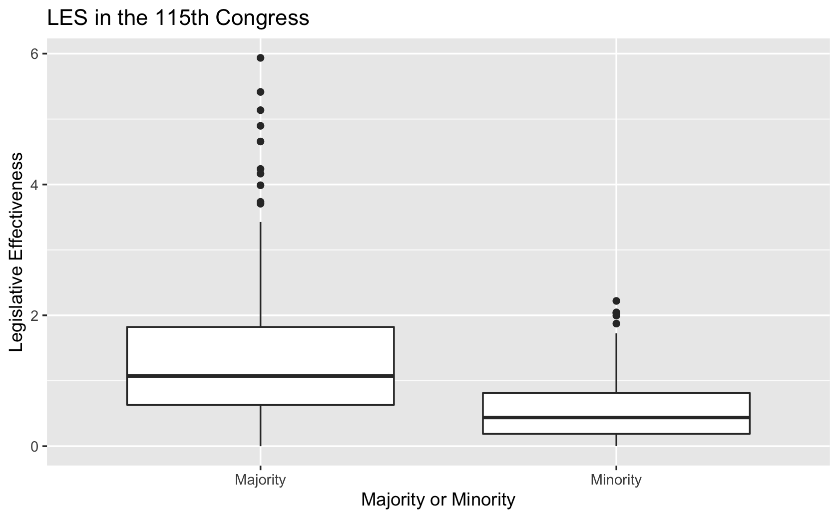
9.4 Practices for week 5
######DO NOT MODIFY. This will load required packages and data.
library(tidyverse)
cces <- drop_na(read_csv(url("https://www.dropbox.com/s/ahmt12y39unicd2/cces_sample_coursera.csv?raw=1")))
#>
#> ── Column specification ─────────────────────────────────────────────
#> cols(
#> .default = col_double()
#> )
#> ℹ Use `spec()` for the full column specifications.Your objective is to replicate these figures, created using the Cooperative Congressional Election Study data. These figures are similar to those we completed in the lecture videos.
cces %>%
  glimpse()
#> Rows: 869
#> Columns: 25
#> $ caseid <dbl> 417614315, 415490556, 414351505, 411855339, 42…
#> $ region <dbl> 3, 1, 3, 1, 2, 1, 2, 1, 3, 3, 1, 3, 4, 3, 2, 4…
#> $ gender <dbl> 1, 2, 2, 2, 1, 1, 2, 1, 1, 2, 2, 1, 1, 2, 2, 1…
#> $ educ <dbl> 2, 6, 3, 5, 3, 2, 3, 5, 6, 2, 3, 6, 3, 3, 6, 3…
#> $ edloan <dbl> 2, 2, 2, 2, 2, 2, 2, 1, 2, 2, 2, 2, 2, 1, 1, 2…
#> $ race <dbl> 1, 1, 2, 6, 1, 1, 1, 1, 1, 1, 1, 1, 3, 2, 1, 1…
#> $ hispanic <dbl> 2, 1, 2, 2, 2, 2, 2, 2, 2, 2, 2, 2, 2, 2, 2, 2…
#> $ employ <dbl> 5, 1, 1, 5, 1, 5, 7, 1, 1, 5, 7, 1, 4, 1, 9, 1…
#> $ marstat <dbl> 3, 1, 4, 3, 1, 5, 1, 1, 5, 4, 1, 1, 5, 2, 1, 5…
#> $ pid7 <dbl> 6, 2, 2, 3, 4, 5, 7, 1, 6, 5, 3, 6, 1, 1, 2, 2…
#> $ ideo5 <dbl> 3, 2, 3, 1, 5, 4, 5, 1, 5, 3, 3, 5, 1, 3, 1, 1…
#> $ pew_religimp <dbl> 1, 3, 1, 2, 4, 3, 1, 4, 4, 1, 2, 1, 3, 2, 2, 4…
#> $ newsint <dbl> 2, 3, 3, 1, 1, 2, 3, 1, 4, 1, 1, 1, 2, 3, 1, 1…
#> $ faminc_new <dbl> 1, 12, 4, 6, 10, 6, 2, 11, 16, 4, 11, 11, 1, 3…
#> $ union <dbl> 3, 3, 3, 2, 1, 3, 3, 2, 3, 3, 3, 3, 3, 2, 3, 3…
#> $ investor <dbl> 2, 2, 1, 1, 2, 1, 2, 1, 2, 2, 1, 1, 2, 1, 1, 1…
#> $ CC18_308a <dbl> 2, 4, 4, 4, 4, 1, 1, 4, 1, 4, 4, 1, 4, 4, 4, 4…
#> $ CC18_310a <dbl> 2, 3, 2, 3, 2, 3, 2, 3, 2, 2, 3, 2, 1, 3, 5, 3…
#> $ CC18_310b <dbl> 3, 2, 2, 3, 2, 3, 2, 3, 3, 3, 3, 2, 1, 5, 3, 3…
#> $ CC18_310c <dbl> 3, 5, 2, 3, 3, 2, 3, 3, 2, 2, 3, 2, 1, 2, 2, 3…
#> $ CC18_310d <dbl> 5, 5, 2, 3, 2, 2, 5, 5, 5, 5, 3, 2, 3, 5, 3, 3…
#> $ CC18_325a <dbl> 1, 2, 1, 2, 1, 1, 1, 2, 2, 2, 2, 1, 2, 2, 2, 2…
#> $ CC18_325b <dbl> 2, 2, 2, 1, 2, 1, 1, 2, 1, 1, 1, 1, 1, 2, 1, 1…
#> $ CC18_325c <dbl> 1, 2, 1, 2, 1, 1, 1, 2, 1, 2, 2, 1, 2, 2, 2, 1…
#> $ CC18_325d <dbl> 1, 1, 2, 1, 1, 1, 1, 1, 2, 1, 2, 1, 2, 1, 2, 1…9.4.1 Exercise 1
Hints:
For the x-axis, use the variable “ideo5.”
Make sure you recode the data for the “ideo5” variable to generate the correct names for the x-axis. You will want to consult the codebook.
Use the fill aesthetic to have R fill in the bars. You do not need to set the colors manually.
Use guides() to drop the legend.
Make sure the axis labels and figure title are correct.
####PUT YOUR CODE HERE
cces %>%
  mutate(
    Ideology = case_when(
      ideo5 == 1 ~ "Very liberal",
      ideo5 == 2 ~ "Liberal",
      ideo5 == 3 ~ "Moderate",
      ideo5 == 4 ~ "Conservative",
      ideo5 == 5 ~ "Very conservative"
    )) %>%
  ggplot(aes(x = Ideology, fill = Ideology)) +
  geom_bar() +
  guides(fill = "none") +
  labs(y = "Count", title = "Respondent Ideology")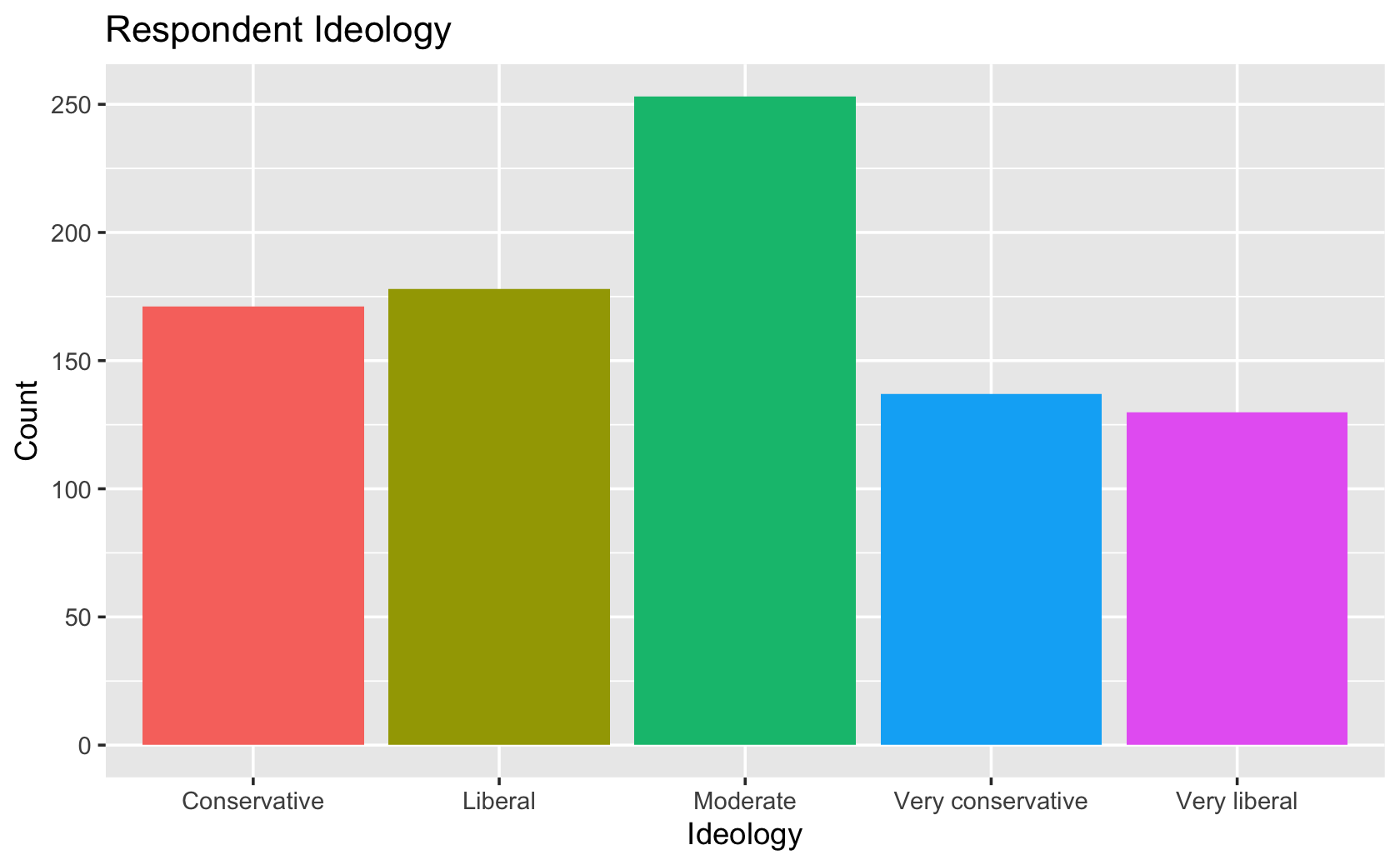
####PUT YOUR CODE HERE
cces %>%
  mutate(
    Ideology = case_when(
      ideo5 == 1 ~ "Very liberal",
      ideo5 == 2 ~ "Liberal",
      ideo5 == 3 ~ "Moderate",
      ideo5 == 4 ~ "Conservative",
      ideo5 == 5 ~ "Very conservative"
    )) %>%
  mutate(Ideology = fct_infreq(Ideology)) %>%
  ggplot(aes(x = Ideology, fill = Ideology)) +
  geom_bar() +
  guides(fill = "none") +
  labs(y = "Count", title = "Respondent Ideology")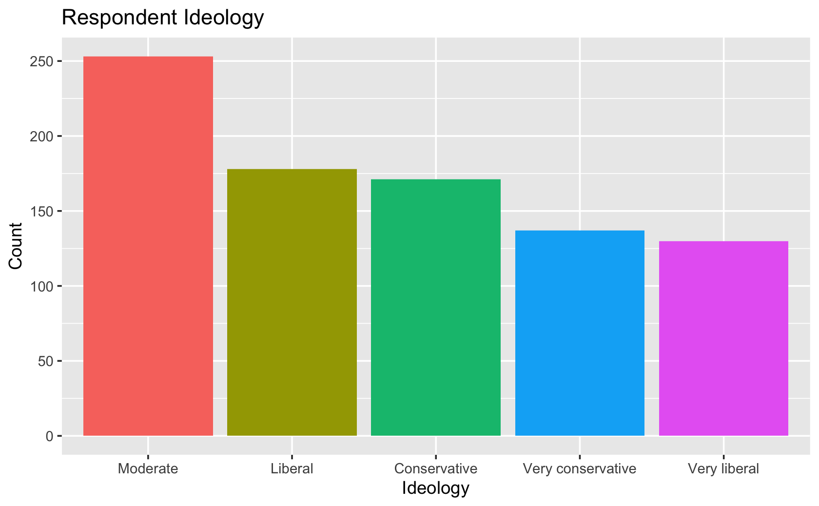
9.4.2 Exercise 2
Hints:
For the x-axis, use the variable “pew_religimp.”
Make sure you recode the data for the “pew_religimp” variable to generate the correct labels for the x-axis. You will want to consult the codebook.
Rename the column for Ideology to make sure the first letter is upper-case (to make the legend appear correctly).
Use the fill aesthetic to have R fill in the bars. You do not need to set the colors manually.
Make sure the axis labels and figure title are correct.
####PUT YOUR CODE HERE
cces %>%
  mutate(
    Ideology = case_when(
      ideo5 == 1 ~ "Very liberal",
      ideo5 == 2 ~ "Liberal",
      ideo5 == 3 ~ "Moderate",
      ideo5 == 4 ~ "Conservative",
      ideo5 == 5 ~ "Very conservative"
    )) %>%
  mutate(
    religion_imp = case_when(
      pew_religimp == 1 ~ "Very imp.",
      pew_religimp == 2 ~ "Somewhat imp.",
      pew_religimp == 3 ~ "Not too imp.",
      pew_religimp == 4 ~ "Not imp."
    )) %>%
  ggplot(aes(x = religion_imp, fill = Ideology)) +
  geom_bar() +
  labs(x = "Importance of Religion",
       y = "Count",
       title = "Importance of Religion by Ideology")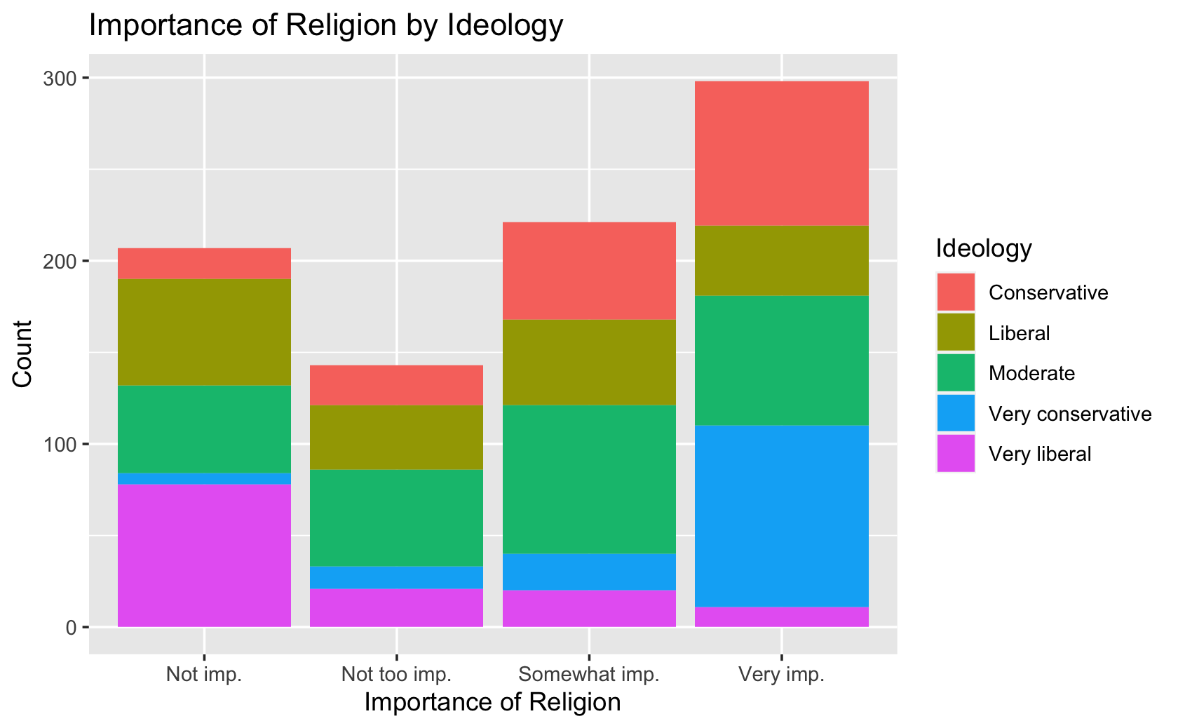
9.4.3 Exercise 3
Instructions:
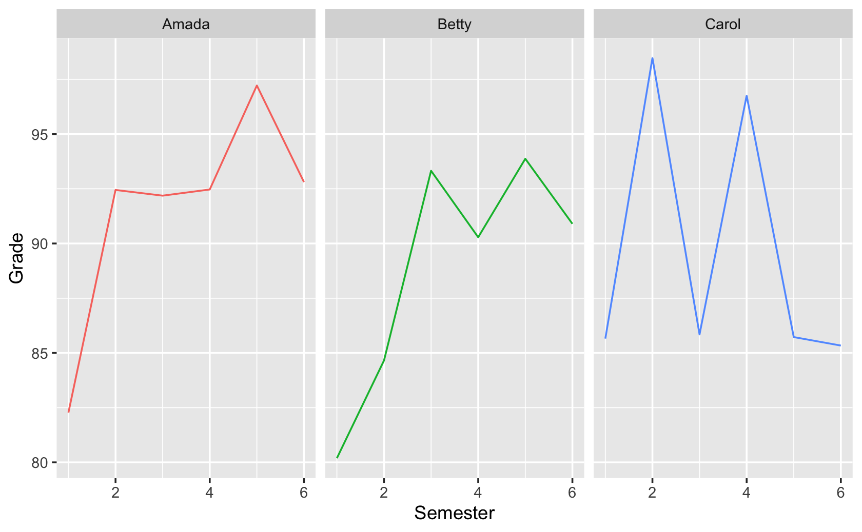
For this visualization, you are creating your own data for practice.
Create a tibble/data frame with three columns: Semester, Student, and Grade.
There should be six semesters and three students (Amanda, Betty, and Carol)
Create grades for the students using the runif() command, with values between 80 and 100. Hint: you’ll need 18 grades total.
The figure should look approximately like this (your vaules will be slightly different):
####PUT YOUR CODE HERE
set.seed(1234)

df <-
  tibble(
    Semester = 1:6 %>% rep(times = 3),
    Student = c("Amada", "Betty", "Carol") %>% rep(each = 6),
    Grade = runif(18, 80, 100)
  )
df
#> # A tibble: 18 x 3
#> Semester Student Grade
#> <int> <chr> <dbl>
#> 1 1 Amada 82.3
#> 2 2 Amada 92.4
#> 3 3 Amada 92.2
#> 4 4 Amada 92.5
#> 5 5 Amada 97.2
#> 6 6 Amada 92.8
#> # … with 12 more rowsdf %>%
ggplot(aes(x = Semester, y = Grade, color = Student)) +
facet_wrap(~ Student) +
geom_line() +
theme(legend.position = "none")