Part 6 Week 3 Synchronous
6.1 Goal
- Go over practices
- Reproducible research
- Relational data
- Strings, regular expression
6.3 Reproducible research
https://bookdown.org/yihui/rmarkdown/basics.html
R Markdown is great for reproducible research: it includes the source code right inside the document, which makes it easy to discover and fix problems, as well as update the output document.
Scientific research that was not done in a reproducible way: e.g., cut-and-paste
The Importance of Reproducible Research in High-Throughput Biology
library(tidyverse)
library(nycflights13)
6.4 Relational data
- Typically you have many tables of data, and you must combine them to answer the questions that you’re interested in.
- Multiple tables of data are called relational data because it is the relations, not just the individual datasets, that are important.
- The most common place to find relational data is in a relational database management system (or RDBMS), a term that encompasses almost all modern databases.
6.4.1 Dataset
We will use the nycflights13 package to learn about relational data.
nycflights13 contains four tibbles that are related to the flights table.
This package provides the following data tables.
?flights: all flights that departed from NYC in 2013 ?weather: hourly meterological data for each airport ?planes: construction information about each plane ?airports: airport names and locations ?airlines: translation between two letter carrier codes and names
flights %>% glimpse()#> Rows: 336,776
#> Columns: 19
#> $ year <int> 2013, 2013, 2013, 2013, 2013, 2013, 2013, 20…
#> $ month <int> 1, 1, 1, 1, 1, 1, 1, 1, 1, 1, 1, 1, 1, 1, 1,…
#> $ day <int> 1, 1, 1, 1, 1, 1, 1, 1, 1, 1, 1, 1, 1, 1, 1,…
#> $ dep_time <int> 517, 533, 542, 544, 554, 554, 555, 557, 557,…
#> $ sched_dep_time <int> 515, 529, 540, 545, 600, 558, 600, 600, 600,…
#> $ dep_delay <dbl> 2, 4, 2, -1, -6, -4, -5, -3, -3, -2, -2, -2,…
#> $ arr_time <int> 830, 850, 923, 1004, 812, 740, 913, 709, 838…
#> $ sched_arr_time <int> 819, 830, 850, 1022, 837, 728, 854, 723, 846…
#> $ arr_delay <dbl> 11, 20, 33, -18, -25, 12, 19, -14, -8, 8, -2…
#> $ carrier <chr> "UA", "UA", "AA", "B6", "DL", "UA", "B6", "E…
#> $ flight <int> 1545, 1714, 1141, 725, 461, 1696, 507, 5708,…
#> $ tailnum <chr> "N14228", "N24211", "N619AA", "N804JB", "N66…
#> $ origin <chr> "EWR", "LGA", "JFK", "JFK", "LGA", "EWR", "E…
#> $ dest <chr> "IAH", "IAH", "MIA", "BQN", "ATL", "ORD", "F…
#> $ air_time <dbl> 227, 227, 160, 183, 116, 150, 158, 53, 140, …
#> $ distance <dbl> 1400, 1416, 1089, 1576, 762, 719, 1065, 229,…
#> $ hour <dbl> 5, 5, 5, 5, 6, 5, 6, 6, 6, 6, 6, 6, 6, 6, 6,…
#> $ minute <dbl> 15, 29, 40, 45, 0, 58, 0, 0, 0, 0, 0, 0, 0, …
#> $ time_hour <dttm> 2013-01-01 05:00:00, 2013-01-01 05:00:00, 2…# airlines: full carrier name from its abbreviated code
airlines %>% glimpse()#> Rows: 16
#> Columns: 2
#> $ carrier <chr> "9E", "AA", "AS", "B6", "DL", "EV", "F9", "FL", "HA…
#> $ name <chr> "Endeavor Air Inc.", "American Airlines Inc.", "Ala…# airports: information about each airport, identified by the faa airport code
airports %>% glimpse()#> Rows: 1,458
#> Columns: 8
#> $ faa <chr> "04G", "06A", "06C", "06N", "09J", "0A9", "0G6", "0G7…
#> $ name <chr> "Lansdowne Airport", "Moton Field Municipal Airport",…
#> $ lat <dbl> 41.13, 32.46, 41.99, 41.43, 31.07, 36.37, 41.47, 42.8…
#> $ lon <dbl> -80.62, -85.68, -88.10, -74.39, -81.43, -82.17, -84.5…
#> $ alt <dbl> 1044, 264, 801, 523, 11, 1593, 730, 492, 1000, 108, 4…
#> $ tz <dbl> -5, -6, -6, -5, -5, -5, -5, -5, -5, -8, -5, -6, -5, -…
#> $ dst <chr> "A", "A", "A", "A", "A", "A", "A", "A", "U", "A", "A"…
#> $ tzone <chr> "America/New_York", "America/Chicago", "America/Chica…# planes: information about each plane, identified by its tailnum
planes %>% glimpse()#> Rows: 3,322
#> Columns: 9
#> $ tailnum <chr> "N10156", "N102UW", "N103US", "N104UW", "N1057…
#> $ year <int> 2004, 1998, 1999, 1999, 2002, 1999, 1999, 1999…
#> $ type <chr> "Fixed wing multi engine", "Fixed wing multi e…
#> $ manufacturer <chr> "EMBRAER", "AIRBUS INDUSTRIE", "AIRBUS INDUSTR…
#> $ model <chr> "EMB-145XR", "A320-214", "A320-214", "A320-214…
#> $ engines <int> 2, 2, 2, 2, 2, 2, 2, 2, 2, 2, 2, 2, 2, 2, 2, 2…
#> $ seats <int> 55, 182, 182, 182, 55, 182, 182, 182, 182, 182…
#> $ speed <int> NA, NA, NA, NA, NA, NA, NA, NA, NA, NA, NA, NA…
#> $ engine <chr> "Turbo-fan", "Turbo-fan", "Turbo-fan", "Turbo-…# weather: weather at each NYC airport for each hour
weather %>% glimpse()#> Rows: 26,115
#> Columns: 15
#> $ origin <chr> "EWR", "EWR", "EWR", "EWR", "EWR", "EWR", "EWR",…
#> $ year <int> 2013, 2013, 2013, 2013, 2013, 2013, 2013, 2013, …
#> $ month <int> 1, 1, 1, 1, 1, 1, 1, 1, 1, 1, 1, 1, 1, 1, 1, 1, …
#> $ day <int> 1, 1, 1, 1, 1, 1, 1, 1, 1, 1, 1, 1, 1, 1, 1, 1, …
#> $ hour <int> 1, 2, 3, 4, 5, 6, 7, 8, 9, 10, 11, 13, 14, 15, 1…
#> $ temp <dbl> 39.02, 39.02, 39.02, 39.92, 39.02, 37.94, 39.02,…
#> $ dewp <dbl> 26.06, 26.96, 28.04, 28.04, 28.04, 28.04, 28.04,…
#> $ humid <dbl> 59.37, 61.63, 64.43, 62.21, 64.43, 67.21, 64.43,…
#> $ wind_dir <dbl> 270, 250, 240, 250, 260, 240, 240, 250, 260, 260…
#> $ wind_speed <dbl> 10.357, 8.055, 11.508, 12.659, 12.659, 11.508, 1…
#> $ wind_gust <dbl> NA, NA, NA, NA, NA, NA, NA, NA, NA, NA, NA, NA, …
#> $ precip <dbl> 0, 0, 0, 0, 0, 0, 0, 0, 0, 0, 0, 0, 0, 0, 0, 0, …
#> $ pressure <dbl> 1012, 1012, 1012, 1012, 1012, 1012, 1012, 1012, …
#> $ visib <dbl> 10, 10, 10, 10, 10, 10, 10, 10, 10, 10, 10, 10, …
#> $ time_hour <dttm> 2013-01-01 01:00:00, 2013-01-01 02:00:00, 2013-…6.4.2 Database schema
The relationships between the different tables
knitr::include_graphics("relational-nycflights.png")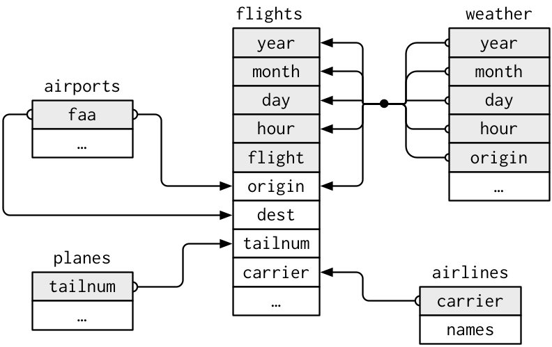
flightsconnects toplanesvia a single variable,tailnum.flightsconnects toairlinesthrough thecarriervariable.flightsconnects toairportsin two ways: via theoriginanddestvariables.flightsconnects toweatherviaorigin(the location), andyear,month,dayandhour(the time).Actual database can be more complicated.
6.4.3 Keys
The variables used to connect each pair of tables are called keys.
A key is a variable (or set of variables) that uniquely identifies an observation.
In simple cases, a single variable is sufficient to identify an observation.
For example, each plane is uniquely identified by its tailnum. In other cases, multiple variables may be needed. For example, to identify an observation in weather you need five variables: year, month, day, hour, and origin.
There are two types of keys:
A primary key uniquely identifies an observation in its own table. planes$tailnum is a primary key because it uniquely identifies each plane in the planes table.
A foreign key uniquely identifies an observation in another table. flights$tailnum is a foreign key because it appears in the flights table where it matches each flight to a unique plane.
# Verify if primary keys uniquely identify each observation
planes %>%
  count(tailnum)
#> # A tibble: 3,322 x 2
#> tailnum n
#> <chr> <int>
#> 1 N10156 1
#> 2 N102UW 1
#> 3 N103US 1
#> 4 N104UW 1
#> 5 N10575 1
#> 6 N105UW 1
#> # … with 3,316 more rowsplanes %>%
count(tailnum) %>%
filter(n > 1)#> # A tibble: 0 x 2
#> # … with 2 variables: tailnum <chr>, n <int>weather %>%
count(year, month, day, hour, origin)#> # A tibble: 26,112 x 6
#> year month day hour origin n
#> <int> <int> <int> <int> <chr> <int>
#> 1 2013 1 1 1 EWR 1
#> 2 2013 1 1 1 JFK 1
#> 3 2013 1 1 1 LGA 1
#> 4 2013 1 1 2 EWR 1
#> 5 2013 1 1 2 JFK 1
#> 6 2013 1 1 2 LGA 1
#> # … with 26,106 more rowsweather %>%
count(year, month, day, hour, origin) %>%
filter(n > 1)#> # A tibble: 3 x 6
#> year month day hour origin n
#> <int> <int> <int> <int> <chr> <int>
#> 1 2013 11 3 1 EWR 2
#> 2 2013 11 3 1 JFK 2
#> 3 2013 11 3 1 LGA 2Sometimes a table doesn’t have an explicit primary key: each row is an observation, but no combination of variables reliably identifies it.
What’s the primary key in the flights table?
flights %>%
  count(year, month, day, flight) %>%
  filter(n > 1)
#> # A tibble: 29,768 x 5
#> year month day flight n
#> <int> <int> <int> <int> <int>
#> 1 2013 1 1 1 2
#> 2 2013 1 1 3 2
#> 3 2013 1 1 4 2
#> 4 2013 1 1 11 3
#> 5 2013 1 1 15 2
#> 6 2013 1 1 21 2
#> # … with 29,762 more rowsflights %>%
count(year, month, day, tailnum) %>%
filter(n > 1)#> # A tibble: 64,928 x 5
#> year month day tailnum n
#> <int> <int> <int> <chr> <int>
#> 1 2013 1 1 N0EGMQ 2
#> 2 2013 1 1 N11189 2
#> 3 2013 1 1 N11536 2
#> 4 2013 1 1 N11544 3
#> 5 2013 1 1 N11551 2
#> 6 2013 1 1 N12540 2
#> # … with 64,922 more rows- surrogate key: If a table lacks a primary key, it’s sometimes useful to add one with eg, row number.
# add one with mutate() and row_number()
flights %>%
  mutate(surrogate_key = row_number()) %>%
  select(surrogate_key, everything())
#> # A tibble: 336,776 x 20
#> surrogate_key year month day dep_time sched_dep_time dep_delay
#> <int> <int> <int> <int> <int> <int> <dbl>
#> 1 1 2013 1 1 517 515 2
#> 2 2 2013 1 1 533 529 4
#> 3 3 2013 1 1 542 540 2
#> 4 4 2013 1 1 544 545 -1
#> 5 5 2013 1 1 554 600 -6
#> 6 6 2013 1 1 554 558 -4
#> # … with 336,770 more rows, and 13 more variables: arr_time <int>,
#> # sched_arr_time <int>, arr_delay <dbl>, carrier <chr>,
#> # flight <int>, tailnum <chr>, origin <chr>, dest <chr>,
#> # air_time <dbl>, distance <dbl>, hour <dbl>, minute <dbl>,
#> # time_hour <dttm>A primary key and the corresponding foreign key in another table form a relation.
- One-to-many. For example, each flight has one plane, but each plane has many flights.
- 1-to-1: think of this as a special case of 1-to-many
- many-to-many: many-to-1 relation plus a 1-to-many relation. For example, each airline flies to many airports; each airport hosts many airlines.
6.4.4 Example of join
flights2 <- flights %>%
  select(year:day, hour, origin, dest, tailnum, carrier)
flights2 %>% head()
#> # A tibble: 6 x 8
#> year month day hour origin dest tailnum carrier
#> <int> <int> <int> <dbl> <chr> <chr> <chr> <chr>
#> 1 2013 1 1 5 EWR IAH N14228 UA
#> 2 2013 1 1 5 LGA IAH N24211 UA
#> 3 2013 1 1 5 JFK MIA N619AA AA
#> 4 2013 1 1 5 JFK BQN N804JB B6
#> 5 2013 1 1 6 LGA ATL N668DN DL
#> 6 2013 1 1 5 EWR ORD N39463 UA6.4.5 How to add full airline name to flights2?
flights2 %>%
  select(-origin, -dest) %>%
  left_join(airlines, by = "carrier")
#> # A tibble: 336,776 x 7
#> year month day hour tailnum carrier name
#> <int> <int> <int> <dbl> <chr> <chr> <chr>
#> 1 2013 1 1 5 N14228 UA United Air Lines Inc.
#> 2 2013 1 1 5 N24211 UA United Air Lines Inc.
#> 3 2013 1 1 5 N619AA AA American Airlines Inc.
#> 4 2013 1 1 5 N804JB B6 JetBlue Airways
#> 5 2013 1 1 6 N668DN DL Delta Air Lines Inc.
#> 6 2013 1 1 5 N39463 UA United Air Lines Inc.
#> # … with 336,770 more rowsx <- tribble(
~key, ~val_x,
1, "x1",
2, "x2",
3, "x3"
)
y <- tribble(
~key, ~val_y,
1, "y1",
2, "y2",
4, "y3"
)
x#> # A tibble: 3 x 2
#> key val_x
#> <dbl> <chr>
#> 1 1 x1
#> 2 2 x2
#> 3 3 x3y#> # A tibble: 3 x 2
#> key val_y
#> <dbl> <chr>
#> 1 1 y1
#> 2 2 y2
#> 3 4 y3knitr::include_graphics("join-outer.png")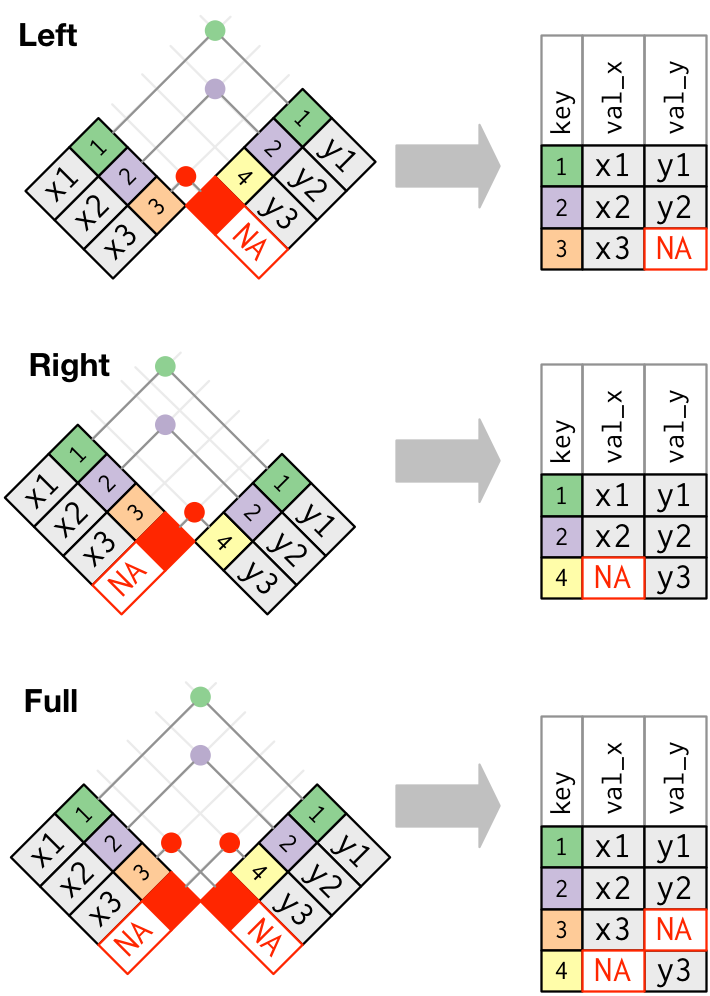
6.4.6 Inner join
An inner join matches pairs of observations whenever their keys are equal and unmatched rows are not included in the result. It’s very possible to lose observations.
x %>%
  inner_join(y, by = "key")
#> # A tibble: 2 x 3
#> key val_x val_y
#> <dbl> <chr> <chr>
#> 1 1 x1 y1
#> 2 2 x2 y26.4.7 Outer joins
6.4.7.1 left join
A left join keeps all observations in x.
x %>%
  left_join(y, by = "key")
#> # A tibble: 3 x 3
#> key val_x val_y
#> <dbl> <chr> <chr>
#> 1 1 x1 y1
#> 2 2 x2 y2
#> 3 3 x3 <NA>6.4.7.2 right join
A right join keeps all observations in y.
x %>%
  right_join(y, by = "key")
#> # A tibble: 3 x 3
#> key val_x val_y
#> <dbl> <chr> <chr>
#> 1 1 x1 y1
#> 2 2 x2 y2
#> 3 4 <NA> y3y %>%
left_join(x, by = "key")#> # A tibble: 3 x 3
#> key val_y val_x
#> <dbl> <chr> <chr>
#> 1 1 y1 x1
#> 2 2 y2 x2
#> 3 4 y3 <NA>6.4.7.3 full join
A full join keeps all observations in x and y.
x %>%
  full_join(y, by = "key")
#> # A tibble: 4 x 3
#> key val_x val_y
#> <dbl> <chr> <chr>
#> 1 1 x1 y1
#> 2 2 x2 y2
#> 3 3 x3 <NA>
#> 4 4 <NA> y36.4.7.4 Duplicate keys
- one-to-many relationship
x <- tribble(
  ~key, ~val_x,
     1, "x1",
     2, "x2",
     2, "x3",
     1, "x4"
)
y <- tribble(
  ~key, ~val_y,
     1, "y1",
     2, "y2"
)

x
#> # A tibble: 4 x 2
#> key val_x
#> <dbl> <chr>
#> 1 1 x1
#> 2 2 x2
#> 3 2 x3
#> 4 1 x4y#> # A tibble: 2 x 2
#> key val_y
#> <dbl> <chr>
#> 1 1 y1
#> 2 2 y2left_join(x, y, by = "key")#> # A tibble: 4 x 3
#> key val_x val_y
#> <dbl> <chr> <chr>
#> 1 1 x1 y1
#> 2 2 x2 y2
#> 3 2 x3 y2
#> 4 1 x4 y16.5 Strings
Regular expressions: a concise language for describing patterns in strings.
string1 <- "This is a string"
string2 <- 'If I want to include a "quote" inside a string, I use single quotes'
special characters
eg, \n, newline, \t, tab, \", ", \', ’
x <- "first line\nsecond line"
cat(x)
#> first line
#> second line# backslash
cat("\" \n \' \t \\")#> "
#> ' \6.5.1 Basic
6.5.1.1 String length
str_length(string1)#> [1] 16str_length(string2)#> [1] 676.5.1.2 Combine string
str_c("x", "y", "z")#> [1] "xyz"str_c("x", "y", sep = ", ")#> [1] "x, y"6.5.1.3 Collapse a vector of strings
str_c(c("x", "y", "z"), collapse = ", ")#> [1] "x, y, z"str_c(c("x", "y", "z"), collapse = "_")#> [1] "x_y_z"6.5.1.4 Subset strings
str_sub(string1, 1, 3)#> [1] "Thi"6.5.1.5 Lower/higher case strings
str_to_lower(string1)#> [1] "this is a string"str_to_upper(string1)#> [1] "THIS IS A STRING"6.5.2 Match
Regexps are a very terse language that allow you to describe patterns in strings.
x <- c("apple", "banana", "pear")
str_view(x, "an")
6.5.2.1 . matches any character
str_view(x, ".a.")6.5.2.2 ^ matches the start
x <- c("apple", "banana", "pear")
str_view(x, "^a")
6.5.2.3 $ matches the end
str_view(x, "a$")6.5.2.4 \d matches any digit
str_view(c("x 1", 67), "\\d")6.5.2.5 \s matches any whitespace
str_view(c("x 1", 67), "\\s")6.5.2.6 [abc] matches a, b, or c
str_view(c("x 1", 67, 'a d', 'ar'), "[abc]")6.5.2.7 [^abc] matches anything except a, b, or c
str_view(c("x 1", 67, 'ac', 'ar'), "[^abc]")6.5.2.8 Repetition, etc
6.6 Factors
Factors are used to work with categorical variables. The first factor is usually used as reference.
x1 <- c("Dec", "Apr", "Jan", "Mar")
sort(x1)
#> [1] "Apr" "Dec" "Jan" "Mar"month_levels <- c(
"Jan", "Feb", "Mar", "Apr", "May", "Jun",
"Jul", "Aug", "Sep", "Oct", "Nov", "Dec"
)
y1 <- factor(x1, levels = month_levels)
y1#> [1] Dec Apr Jan Mar
#> Levels: Jan Feb Mar Apr May Jun Jul Aug Sep Oct Nov Dec