Part 3 Week 1 Asynchronous
Getting Started with Data Visualization in R > Week 1
3.1 Installing R and Getting Started
3.2 R basics
3.2.1 Basic R
####Do Basic Math

2 + 2
#> [1] 42 - 2#> [1] 02 / 2#> [1] 12 * 2#> [1] 4a <- 2 + 2
####Run each line by either (1) setting the cursor at the end of the line and hitting control+enter on a PC or cmd+enter on Mac or click in the run button in the menu bar above or (2) selecting the line(s) of code you want to execute and then using the keyboard short cut or clicking run
##### You can use pound signs/hashtags to tell R to ignore lines of code
#2+2
2 + 2#> [1] 4#############
#START FOLLOWING ALONG WITH THE VIDEO HERE
#############
##### If you tell R to do something it doesn't understand, it will throw an error. R is very picky about punctuation, spelling etc.
######these commands will not do anything
#2234r*S&F(SD&F234)
#c(c))
#### R can also act do logical tests using logical operators.
####Is equal?
2 == 2#> [1] TRUE2 == 3#> [1] FALSE#####Is not equal?
2 != 2#> [1] FALSE2 != 3#> [1] TRUE####Greater than and less than
2 > 1#> [1] TRUE2 < 1#> [1] FALSE####Greater than or equal to, less than or equal to
3 >= 1#> [1] TRUE3 <= 1#> [1] FALSE#### R can work with character strings
"apple"#> [1] "apple"#### It is ok to use spaces in character strings.
"an apple"#> [1] "an apple"###You can use logical operators to see whether character strings exactly match each other
"apple" == "apple"#> [1] TRUE"apple" == "appla"#> [1] FALSE"apple" == "orange"#> [1] FALSE"apple" != "orange"#> [1] TRUE#### If you try to use inequalities with characters, R will compare how long the character string is
"apple" < "apples"#> [1] TRUE"apple" > "apples"#> [1] FALSE####save the output of a command to an object
a <- 2 + 2
my_a <- 2 + 2
my.a <- 2 + 2
######## Don't do this. It won't work
#9a <- 2+2
#my object <- 2+2
#### See what is in the object by "running" the object
a#> [1] 4####you can save series of numbers or strings and put them into vectors using the combine function, c().
numbers <- c(1, 2, 3)
numbers#> [1] 1 2 3fruits <- c("apple", "orange")
fruits#> [1] "apple" "orange"numbers2 <- c(4:6)
numbers2#> [1] 4 5 6true_false <- c(TRUE, FALSE, TRUE)
true_false#> [1] TRUE FALSE TRUE#### You can combine vectors together
numbers3 <- c(7:9)
all_numbers <- c(numbers, numbers2, numbers3)
all_numbers#> [1] 1 2 3 4 5 6 7 8 9#####You can select certain elements of a vector
x <- c(-1, 10, 11, 12, 13, 14, 15, 16, 17, 18, 19)
### By position in the vector
x[4] #The fourth element.#> [1] 12x[-4] #All but the fourth.#> [1] -1 10 11 13 14 15 16 17 18 19x[2:4] #Elements two to four.#> [1] 10 11 12x[-(2:4)] #All elements except two to four.#> [1] -1 13 14 15 16 17 18 19x[c(1, 5)] #Elements one and five.#> [1] -1 13### By Value
x[x == 10] # Elements which are equal to 10.#> [1] 10x[x < 0] #all elements less than zero.#> [1] -1x[x %in% c(10, 12, 15)] #Elements in the set 2, 4, 7.#> [1] 10 12 15#### When you save different kinds of data, that data is given a "class" that describes what kind of data are in the vector
class(numbers)#> [1] "numeric"class(fruits)#> [1] "character"class(true_false)#> [1] "logical"#### If you combine numbers and character vectors together, the numbers will convert to characters
fruits_numbers <- c(numbers, fruits)
fruits_numbers#> [1] "1" "2" "3" "apple" "orange"#### Generally for data visualization purposes, it is good to not mix characters and numbers in the same vector.
##### You can change the class of a vector using as.logical,as.numeric,as.character, and as.factor
####here's an example with 1s and 0s
my_vector <- c(1, 0, 1, 0)
my_vector_character <- as.character(my_vector)
my_vector_character#> [1] "1" "0" "1" "0"class(my_vector_character)#> [1] "character"my_vector_logical <- as.logical(my_vector)
my_vector_logical#> [1] TRUE FALSE TRUE FALSEclass(my_vector_logical)#> [1] "logical"my_vector_factor <- as.factor(my_vector)
my_vector_factor#> [1] 1 0 1 0
#> Levels: 0 1class(my_vector_factor)#> [1] "factor"my_vector_numeric_again <- as.numeric(my_vector_character)
my_vector_numeric_again#> [1] 1 0 1 0class(my_vector_numeric_again)#> [1] "numeric"3.2.2 Functions in R
####Functions

add <- function(x, y) {
  x + y
}

add(2, 3)
#> [1] 5####The last expression is returned
add_and_multiply_version1 <- function(x, y) {
x + y
x * y
}
add_and_multiply_version1(2, 3)#> [1] 6####you can force R to return a specific object
add_and_multiply_version2 <- function(x, y) {
total <- x + y
product <- x * y
total_and_product <- c(total, product)
subtract <- x - y
return(total_and_product)
}
add_and_multiply_version2(2, 3)#> [1] 5 6##### R has many basic mathematical functions already built in that can be applied to numbers and vectors of numbers
###add two or more numbers
sum(c(2, 3, 5))#> [1] 10####add all the numbers in two vectors
sum(c(1, 2, 3), c(4, 5))#> [1] 15#####this does the same thing, just saving the vector to an object
my_vector <- c(1, 2, 3, 4, 5)
sum(my_vector)#> [1] 15##### There are many other functions for doing basic math and descriptive statistics
max(my_vector)#> [1] 5min(my_vector)#> [1] 1median(my_vector)#> [1] 3mean(my_vector)#> [1] 3sd(my_vector) ###standard deviation#> [1] 1.581summary(my_vector) ### a five number summary#> Min. 1st Qu. Median Mean 3rd Qu. Max.
#> 1 2 3 3 4 5##### Other functions will sort vectors or tell you information about the vector
my_vector <- c(2, 2, 1, 3, 5)
sort(my_vector)#> [1] 1 2 2 3 5rev(my_vector)#> [1] 5 3 1 2 2table(my_vector)#> my_vector
#> 1 2 3 5
#> 1 2 1 1unique(my_vector)#> [1] 2 1 3 5length(my_vector)#> [1] 5####create data fast
seq(1, 5)#> [1] 1 2 3 4 5seq(1, 9, by = 2)#> [1] 1 3 5 7 9rep("a", 5)#> [1] "a" "a" "a" "a" "a"rep(10, 5)#> [1] 10 10 10 10 103.3 Dataframe
#####creating dataframes

variable1 <- c(1, 2, 3, 4, 5)
variable2 <- c(6, 7, 8, 9, 10)

data.frame(variable1, variable2)
#> variable1 variable2
#> 1 1 6
#> 2 2 7
#> 3 3 8
#> 4 4 9
#> 5 5 10my_dat <- data.frame("height" = variable1, "weight" = variable2)
my_dat#> height weight
#> 1 1 6
#> 2 2 7
#> 3 3 8
#> 4 4 9
#> 5 5 10#####get a single column of a dataframe
my_dat$weight#> [1] 6 7 8 9 10####use a column in a function
mean(my_dat$weight)#> [1] 8####save a column to another object
my_weights <- my_dat$weight
my_weights#> [1] 6 7 8 9 10####selecting data from dataframes
#####remember you specify row, then column in the brackets
###first row, all columns
my_dat[1, ]#> height weight
#> 1 1 6###first column, all rows
my_dat[, 1]#> [1] 1 2 3 4 5###first column, first row,
my_dat[1, 1]#> [1] 1###first column, first three rows
my_dat[1:3, 1]#> [1] 1 2 3#####creating new columns
####single value repeated
my_dat$variable3 <- 100
my_dat#> height weight variable3
#> 1 1 6 100
#> 2 2 7 100
#> 3 3 8 100
#> 4 4 9 100
#> 5 5 10 100####add vector with same length
my_dat$variable4 <- c("apple", "orange", "grape", "cherry", "melon")
my_dat#> height weight variable3 variable4
#> 1 1 6 100 apple
#> 2 2 7 100 orange
#> 3 3 8 100 grape
#> 4 4 9 100 cherry
#> 5 5 10 100 melon####this won't work because the vector is too short - needs to be same length as other vectors/columns in the dataframe
#my_dat$variable5 <- c("banana","mango")
####get the dimensions of a dataframe (rows and columns)
dim(my_dat)#> [1] 5 4####get more information about the structure of a data frame
str(my_dat)#> 'data.frame': 5 obs. of 4 variables:
#> $ height : num 1 2 3 4 5
#> $ weight : num 6 7 8 9 10
#> $ variable3: num 100 100 100 100 100
#> $ variable4: chr "apple" "orange" "grape" "cherry" ...nrow(my_dat)#> [1] 5ncol(my_dat)#> [1] 4###get the column headers of the data frame
names(my_dat)#> [1] "height" "weight" "variable3" "variable4"###if you have a big dataframe, use head() to see the first few rows or tail to see the last few
head(my_dat)#> height weight variable3 variable4
#> 1 1 6 100 apple
#> 2 2 7 100 orange
#> 3 3 8 100 grape
#> 4 4 9 100 cherry
#> 5 5 10 100 melontail(my_dat)#> height weight variable3 variable4
#> 1 1 6 100 apple
#> 2 2 7 100 orange
#> 3 3 8 100 grape
#> 4 4 9 100 cherry
#> 5 5 10 100 melon####Spreadsheet View
# View(my_dat)
#####Missing data causes lots of problems. Some functions "break" and throw errors if you include missing data
with_missing <- c(1, 2, 3, NA)
sum(with_missing)#> [1] NA#### You should look at the documentation for a function to understand how it handles missing data. Sometimes you can use an argument with a function to tell it how to deal with the missing data, often telling the function to ignore the missing cells.
# ?sum
sum(with_missing, na.rm = TRUE)#> [1] 6#####combining two dataframes with cbind
my_dat2 <- data.frame("variable4" = 400:499, "variable5" = 500:599)
all_dat <- cbind(my_dat, my_dat2)
head(all_dat)#> height weight variable3 variable4 variable4 variable5
#> 1 1 6 100 apple 400 500
#> 2 2 7 100 orange 401 501
#> 3 3 8 100 grape 402 502
#> 4 4 9 100 cherry 403 503
#> 5 5 10 100 melon 404 504
#> 6 1 6 100 apple 405 505#### adding a row
new_row <- c(1000, 2000, 3000, 4000)
all_dat_plus_new_row <- rbind(all_dat, new_row)
tail(all_dat_plus_new_row)#> height weight variable3 variable4 variable4 variable5
#> 96 1 6 100 apple 495 595
#> 97 2 7 100 orange 496 596
#> 98 3 8 100 grape 497 597
#> 99 4 9 100 cherry 498 598
#> 100 5 10 100 melon 499 599
#> 101 1000 2000 3000 4000 1000 2000#### combining two dataframes with rbind
#####you have to make sure the two dataframes have the same column names and order
#######this won't work
# my_dat <- data.frame("variable1"=1:100,"variable2"=200:299)
# my_dat2 <- data.frame("variable4"=400:499,"variable5"=500:599)
# rbind(my_dat,my_dat2)
######this will work
my_dat <- data.frame("variable1" = 1:100, "variable2" = 200:299)
my_dat2 <- data.frame("variable1" = 400:499, "variable2" = 500:599)
rbind(my_dat, my_dat2)#> variable1 variable2
#> 1 1 200
#> 2 2 201
#> 3 3 202
#> 4 4 203
#> 5 5 204
#> 6 6 205
#> 7 7 206
#> 8 8 207
#> 9 9 208
#> 10 10 209
#> 11 11 210
#> 12 12 211
#> 13 13 212
#> 14 14 213
#> 15 15 214
#> 16 16 215
#> 17 17 216
#> 18 18 217
#> 19 19 218
#> 20 20 219
#> 21 21 220
#> 22 22 221
#> 23 23 222
#> 24 24 223
#> 25 25 224
#> 26 26 225
#> 27 27 226
#> 28 28 227
#> 29 29 228
#> 30 30 229
#> 31 31 230
#> 32 32 231
#> 33 33 232
#> 34 34 233
#> 35 35 234
#> 36 36 235
#> 37 37 236
#> 38 38 237
#> 39 39 238
#> 40 40 239
#> 41 41 240
#> 42 42 241
#> 43 43 242
#> 44 44 243
#> 45 45 244
#> 46 46 245
#> 47 47 246
#> 48 48 247
#> 49 49 248
#> 50 50 249
#> 51 51 250
#> 52 52 251
#> 53 53 252
#> 54 54 253
#> 55 55 254
#> 56 56 255
#> 57 57 256
#> 58 58 257
#> 59 59 258
#> 60 60 259
#> 61 61 260
#> 62 62 261
#> 63 63 262
#> 64 64 263
#> 65 65 264
#> 66 66 265
#> 67 67 266
#> 68 68 267
#> 69 69 268
#> 70 70 269
#> 71 71 270
#> 72 72 271
#> 73 73 272
#> 74 74 273
#> 75 75 274
#> 76 76 275
#> 77 77 276
#> 78 78 277
#> 79 79 278
#> 80 80 279
#> 81 81 280
#> 82 82 281
#> 83 83 282
#> 84 84 283
#> 85 85 284
#> 86 86 285
#> 87 87 286
#> 88 88 287
#> 89 89 288
#> 90 90 289
#> 91 91 290
#> 92 92 291
#> 93 93 292
#> 94 94 293
#> 95 95 294
#> 96 96 295
#> 97 97 296
#> 98 98 297
#> 99 99 298
#> 100 100 299
#> 101 400 500
#> 102 401 501
#> 103 402 502
#> 104 403 503
#> 105 404 504
#> 106 405 505
#> 107 406 506
#> 108 407 507
#> 109 408 508
#> 110 409 509
#> 111 410 510
#> 112 411 511
#> 113 412 512
#> 114 413 513
#> 115 414 514
#> 116 415 515
#> 117 416 516
#> 118 417 517
#> 119 418 518
#> 120 419 519
#> 121 420 520
#> 122 421 521
#> 123 422 522
#> 124 423 523
#> 125 424 524
#> 126 425 525
#> 127 426 526
#> 128 427 527
#> 129 428 528
#> 130 429 529
#> 131 430 530
#> 132 431 531
#> 133 432 532
#> 134 433 533
#> 135 434 534
#> 136 435 535
#> 137 436 536
#> 138 437 537
#> 139 438 538
#> 140 439 539
#> 141 440 540
#> 142 441 541
#> 143 442 542
#> 144 443 543
#> 145 444 544
#> 146 445 545
#> 147 446 546
#> 148 447 547
#> 149 448 548
#> 150 449 549
#> 151 450 550
#> 152 451 551
#> 153 452 552
#> 154 453 553
#> 155 454 554
#> 156 455 555
#> 157 456 556
#> 158 457 557
#> 159 458 558
#> 160 459 559
#> 161 460 560
#> 162 461 561
#> 163 462 562
#> 164 463 563
#> 165 464 564
#> 166 465 565
#> 167 466 566
#> 168 467 567
#> 169 468 568
#> 170 469 569
#> 171 470 570
#> 172 471 571
#> 173 472 572
#> 174 473 573
#> 175 474 574
#> 176 475 575
#> 177 476 576
#> 178 477 577
#> 179 478 578
#> 180 479 579
#> 181 480 580
#> 182 481 581
#> 183 482 582
#> 184 483 583
#> 185 484 584
#> 186 485 585
#> 187 486 586
#> 188 487 587
#> 189 488 588
#> 190 489 589
#> 191 490 590
#> 192 491 591
#> 193 492 592
#> 194 493 593
#> 195 494 594
#> 196 495 595
#> 197 496 596
#> 198 497 597
#> 199 498 598
#> 200 499 5993.4 Basics of Importing Data into R
####Importing Data in R

####Import CSV
cces_sample <-
  read.csv("/Users/haoqiwang/Desktop/2021REUDataScience/week1/cces_sample_coursera.csv")

####Write CSV
write.csv(cces_sample,
          "/Users/haoqiwang/Desktop/2021REUDataScience/week1/test.csv")

####type in your directory path in setwd() or use the Session-->Set Working Directory menu options

getwd()
#> [1] "/Users/haoqiwang/Desktop/2021REUDataScience"setwd("/Users/haoqiwang/Desktop/2021REUDataScience/week1")
#### Don't need the whole file path now
cces_sample <- read.csv("cces_sample_coursera.csv")
class(cces_sample)#> [1] "data.frame"median(cces_sample$pew_religimp, na.rm = T)#> [1] 2table(cces_sample$race)#>
#> 1 2 3 4 5 6 7 8
#> 794 81 67 27 6 14 10 13.5 Base R Visualizations
#####Visualizations with Base R

####Univariate Statistics

numbers1 <- c(1, 1, 1, 2, 2, 3, 3, 3, 4, 4, 4, 4, 5, 5, 5, 5, 6, 6, 6)

hist(numbers1)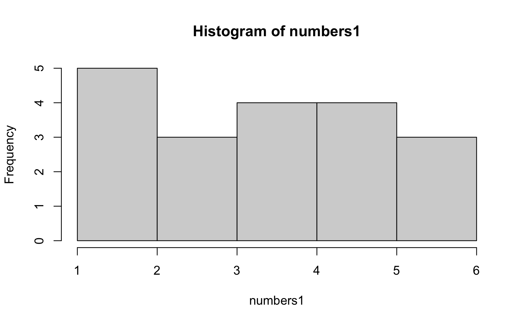
boxplot(numbers1)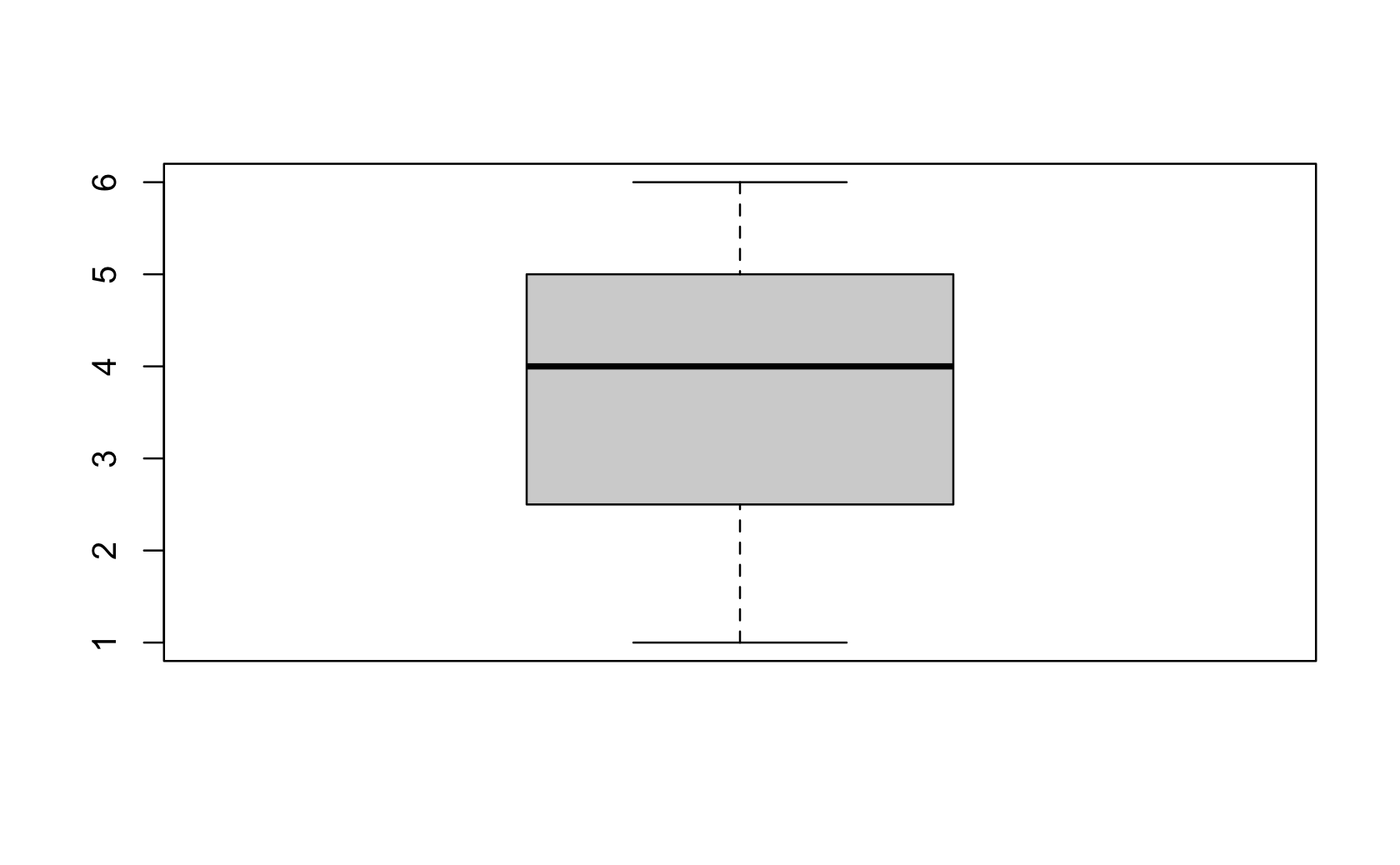
numbers2 <- c(5, 5, 5, 5, 5, 6, 6, 6, 7, 7, 7, 8, 8, 8, 9, 9, 9)

boxplot(numbers1, numbers2)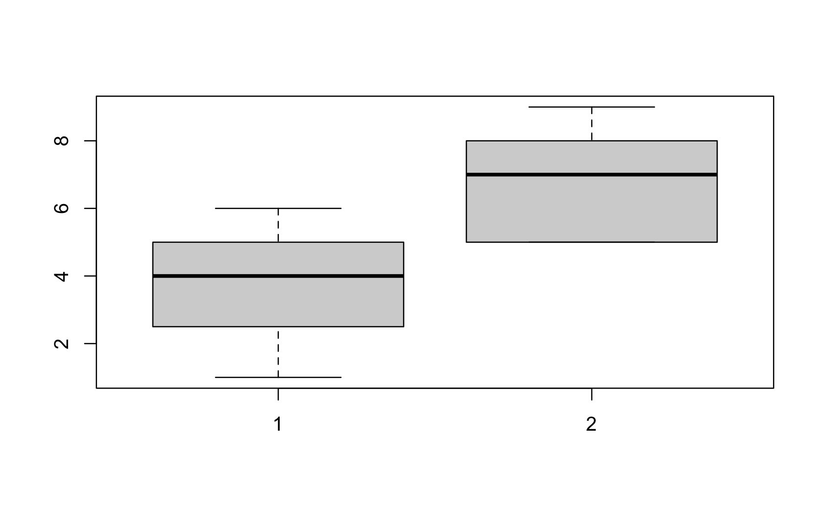
######Bivariate Statistics

#####make some fake data to create a scatterplot

#rnorm - normal distribution
#rpois - poisson
#rbinom - binomial
#runif - uniform

variable1 <- runif(50, 0, 100)
variable2 <- runif(50, 0, 100)
my_dat <- data.frame(variable1, variable2)

#####this does the same thing as the previous three lines
my_dat <-
  data.frame("variable1" = runif(50, 0, 100),
             "variable2" = runif(50, 0, 100))

#### Scatterplot
plot(my_dat$variable1, my_dat$variable2)

#####this does the same thing
plot(x = my_dat$variable1, y = my_dat$variable2)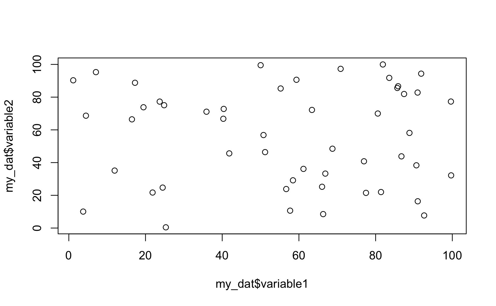
###Base R has some limited graphics customization ability
plot(
  my_dat$variable1,
  my_dat$variable2,
  main = "My First Plot",
  ###add main title
  xlab = "Variable 1",
  ### x axis label
  ylab = "Variable 2",
  ### y axis label
  ylim = c(0, 150),
  xlim = c(0, 150)
)### set the length of the x and y axes.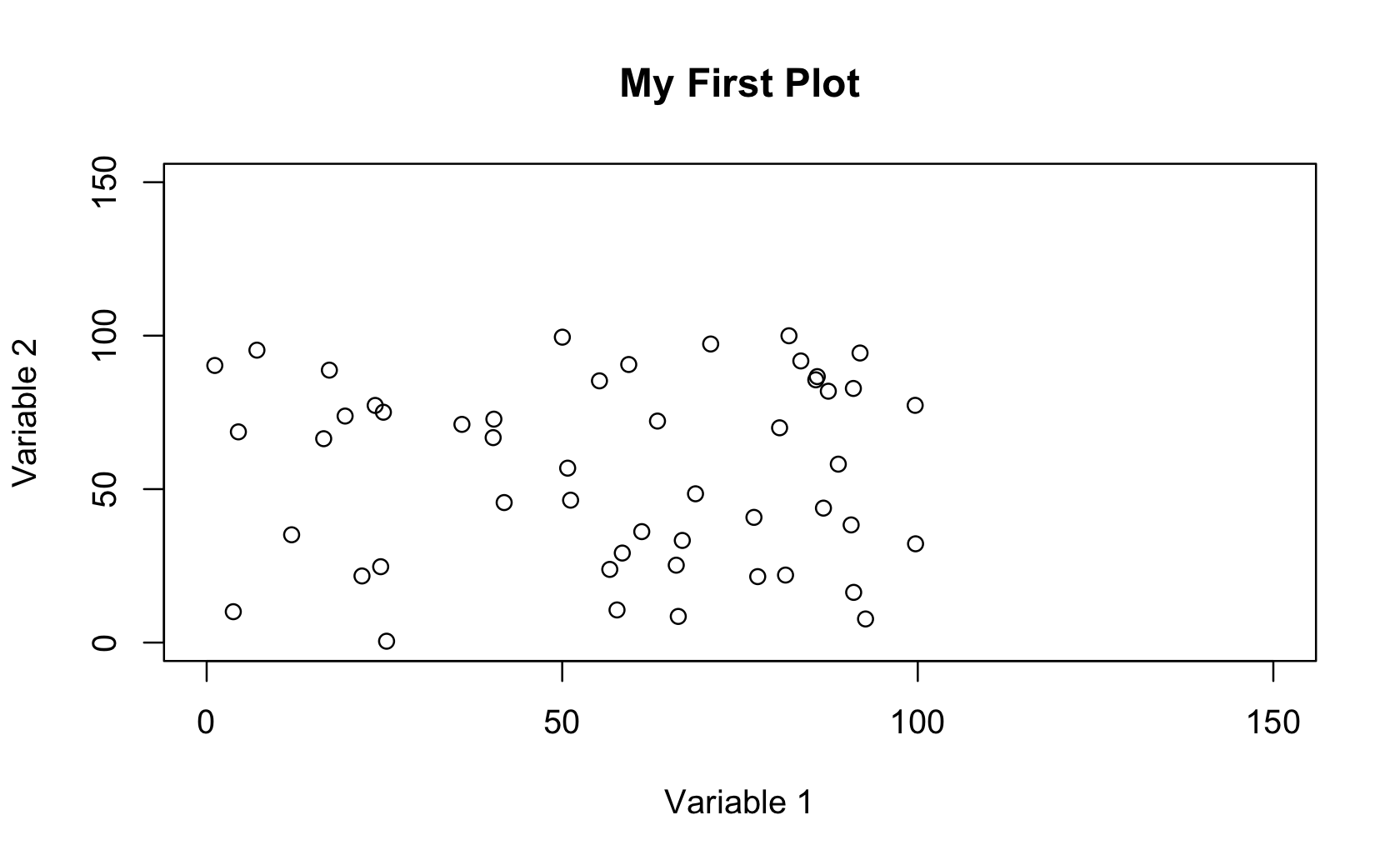
# ? plot3.6 Practices
# Problem 1

# Create a data frame that includes two columns, one named "Animals" and the other named "Foods". The first column should be this vector (note the intentional repeated values): Dog, Cat, Fish, Fish, Lizard


#The second column should be this vector: Bread, Orange, Chocolate, Carrots, Milk


#### Write your code below:

Animals <- c("Dog", "Cat", "Fish", "Fish", "Lizard")
Foods <- c("Bread", "Orange", "Chocolate", "Carrots", "Milk")
df <- data.frame(Animals, Foods)
df
#> Animals Foods
#> 1 Dog Bread
#> 2 Cat Orange
#> 3 Fish Chocolate
#> 4 Fish Carrots
#> 5 Lizard Milk# Problem 2
# Using the data frame created in Problem 2, use the table() command to create a frequency table for the column called "Animals".
#### Write your code below:
table(df$Animals)#>
#> Cat Dog Fish Lizard
#> 1 1 2 1# Problem 3
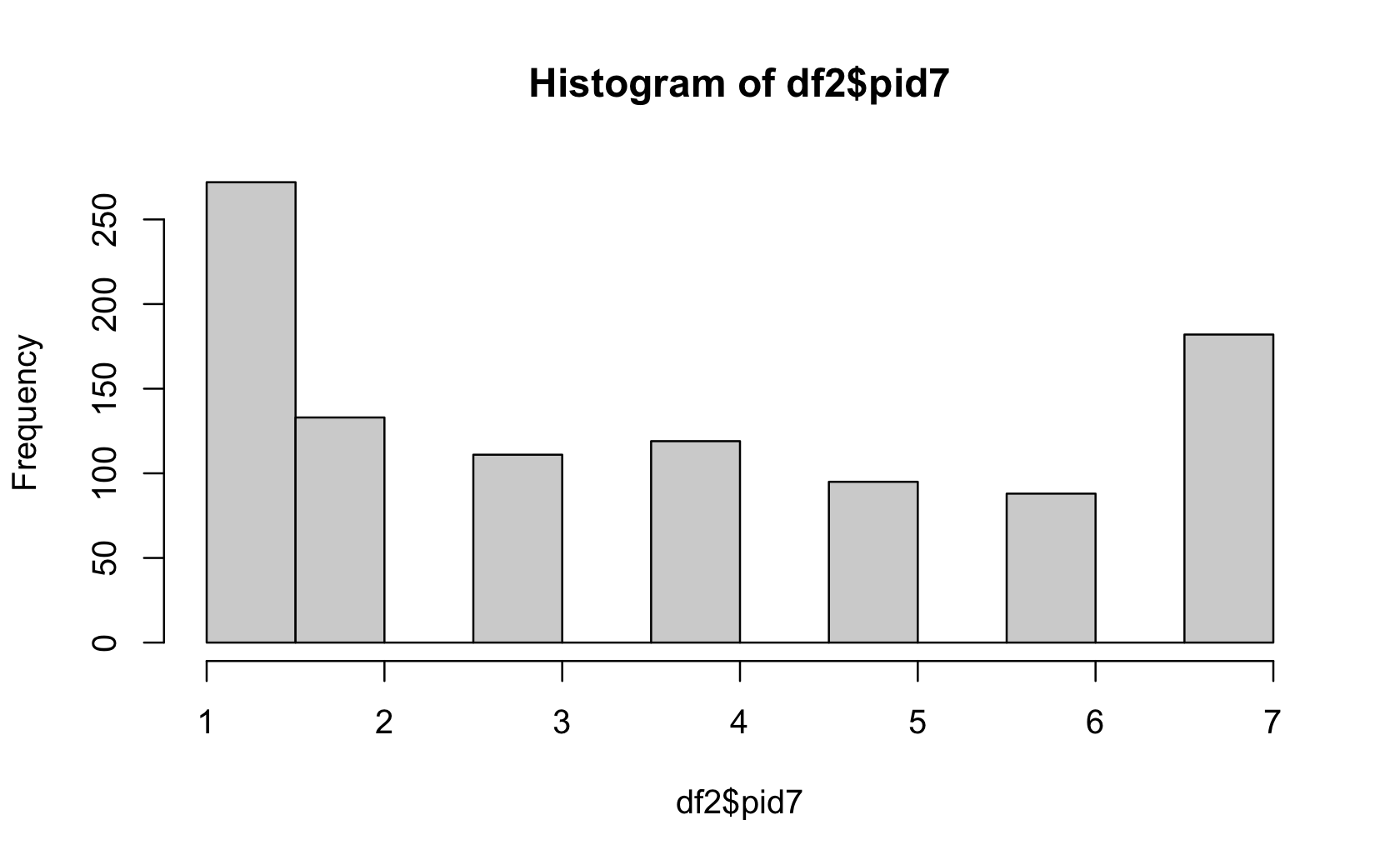
# Use read.csv() to import the survey data included in this assignment. Using that data, make a histogram of the column called "pid7".
#### Write your code below:
df2 <- read.csv("week1/cces_sample_coursera.csv")hist(df2$pid7)